Ch. 16: Dates and times

Key questions:

16.2.4. #3
16.3.4. #1, 4, 5
16.4.5. #4

Functions and notes:

today get current date
now get current date-time
ymd_hms one example of straight-forward set-of of functions that take either strings or unquoted numbers and output dates or date-times
make_datetime create date-time from individual components, e.g. make_datetime(year, month, day, hour, minute)
as_date_time and as_date let you switch between date-time and dates, e.g. as_datetime(today()) or as_date(now())
Accessor functions let you pull out components from an existing date-time:
- year, month, mday, yday, wday, hour, minute, second
  - month and wday have label = TRUE to pull the abbreviated name rather than the number, and pull full name with abbr = FALSE
- You can also use these to set particular components year(datetime) <- 2020
update allows you to specify multiple values at one time, e.g. update(datetime, year = 2020, month = 2, mday = 2, hour = 2)
- When values are too big they roll-over e.g. update(ymd("2015-02-01"), mday = 30) will become ‘2015-03-02’
Rounding functions to nearest unit of time
- floor_date, round_date, ceiling_date
as.duration convert diff-time to a duration
Durations (can add and multiply):
- dseconds, dhours, ddays, dweeks, dyears
Periods (can add and multiply), more likely to do what you expect than duration:
- seconds, minutes, hours, days, weeks, months
Interval is a duration with a starting point, making it precise and possible to determine EXACT length
- e.g. (today() %--% next_year) / ddays(1) to find exact duration
Sys.timezone to see what R thinks your current time zone is
tz = arg in ymd_hms let’s you change printing behavior (not underlying value, as assumes UTC unless changed)
with_tz allows you to print an existing date-time object to a specific other timezone
force_tz when have an object that’s been labeled with wrong time-zone and need to fix it

16.2: Creating date/times

Note that 1 in date-times is treated as 1 - second in numeric contexts, so example below sets binwidth = 86400 to specify 1 day

make_datetime_100 <- function(year, month, day, time) {
  make_datetime(year, month, day, time %/% 100, time %% 100)
}

flights_dt <- flights %>% 
  filter(!is.na(dep_time), !is.na(arr_time)) %>% 
  mutate_at(c("dep_time", "arr_time", "sched_dep_time", "sched_arr_time"), ~make_datetime_100(year, month, day, .)) %>% 
  select(origin, dest, ends_with("delay"), ends_with("time"))

flights_dt %>% 
  ggplot(aes(dep_time)) + 
  geom_freqpoly(binwidth = 86400)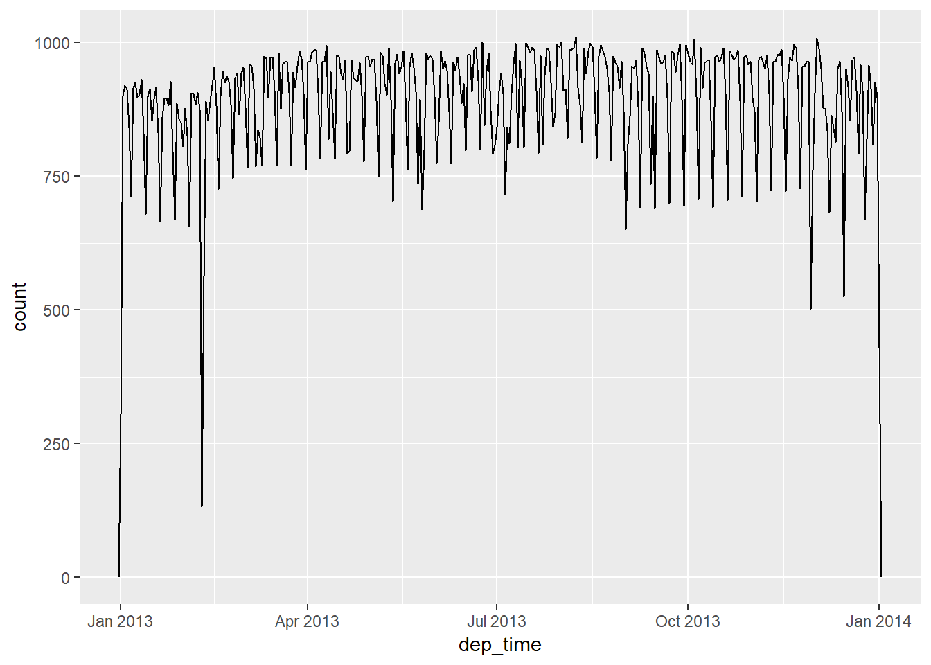

16.2.4

What happens if you parse a string that contains invalid dates?
```
ymd(c("2010-10-10", "bananas"))
```
```
## Warning: 1 failed to parse.
```
```
## [1] "2010-10-10" NA
```
- Outputs an NA and sends warning of number that failed to parse
What does the tzone argument to today() do? Why is it important?
- Let’s you specify timezones, may be different days depending on location
```
today(tzone = "MST")
```
```
## [1] "2019-06-05"
```
```
now(tzone = "MST")
```
```
## [1] "2019-06-05 16:27:06 MST"
```

Use the appropriate lubridate function to parse each of the following dates:

d1 <- "January 1, 2010"
d2 <- "2015-Mar-07"
d3 <- "06-Jun-2017"
d4 <- c("August 19 (2015)", "July 1 (2015)")
d5 <- "12/30/14" # Dec 30, 2014

mdy(d1)

## [1] "2010-01-01"

ymd(d2)

## [1] "2015-03-07"

dmy(d3)

## [1] "2017-06-06"

mdy(d4)

## [1] "2015-08-19" "2015-07-01"

mdy(d5)

## [1] "2014-12-30"

16.3: Date-time components

This allows you to plot the number of flights per week

flights_dt %>% 
  count(week = floor_date(dep_time, "week")) %>% 
  ggplot(aes(week, n)) +
    geom_line()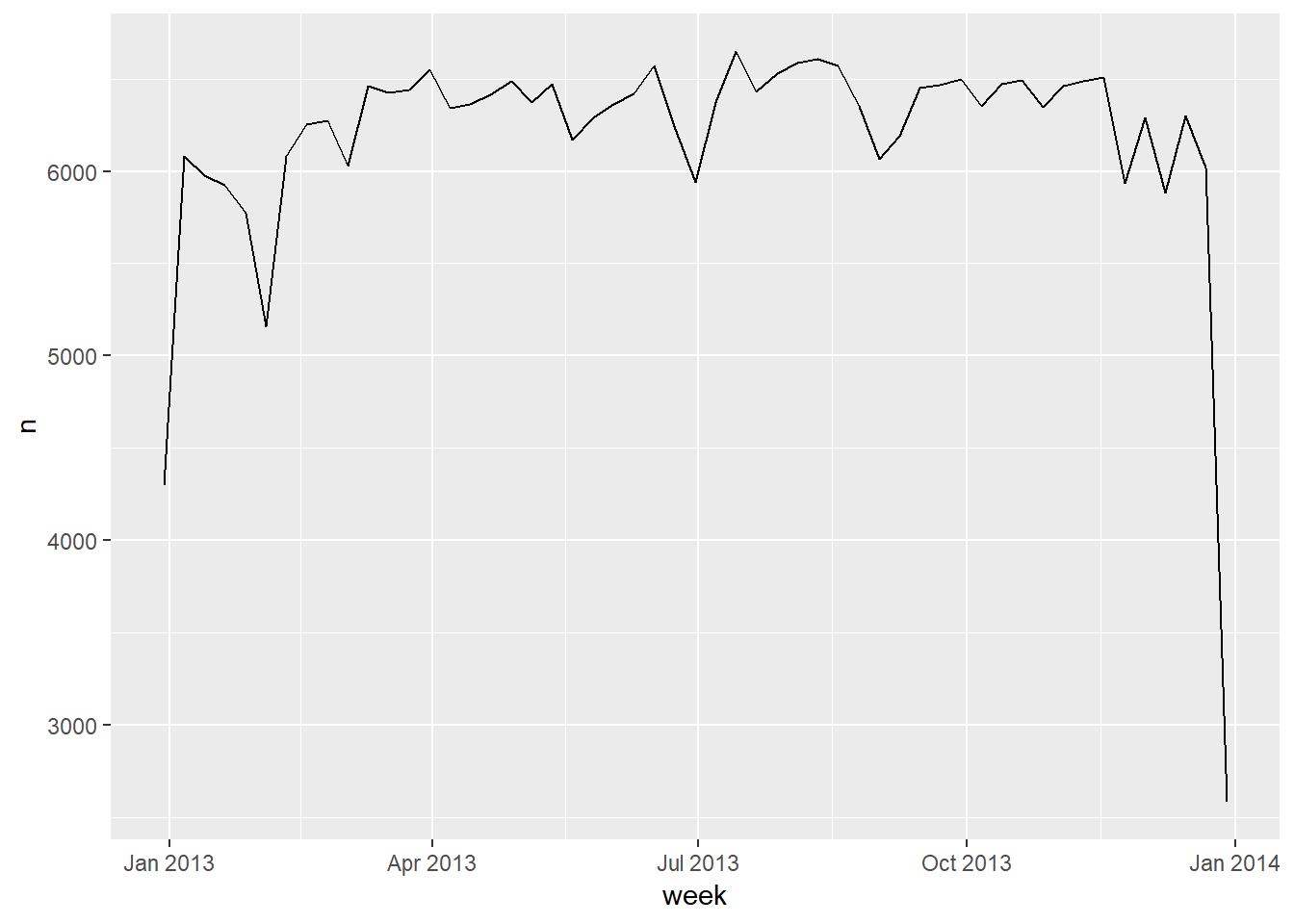

16.3.4

How does the distribution of flight times within a day change over the course of the year?

Median flight time by day

flights_dt %>%
  transmute(quarter_dep = quarter(dep_time) %>% factor(),
            day_dep = as_date(dep_time),
            dep_time = as.hms(dep_time)) %>% 
  group_by(quarter_dep, day_dep) %>% 
  summarise(day_median = median(dep_time)) %>% 
  ungroup() %>% 
  ggplot(aes(x = day_dep, y = day_median)) +
  geom_line(aes(colour = quarter_dep, group = 1)) +
  labs(title = "Median flight times by day, coloured by quarter", subtitle = "Typical flight times change with daylight savings times")+
  geom_vline(xintercept = ymd("20130310"), linetype = 2)+
  geom_vline(xintercept = ymd("20131103"), linetype = 2)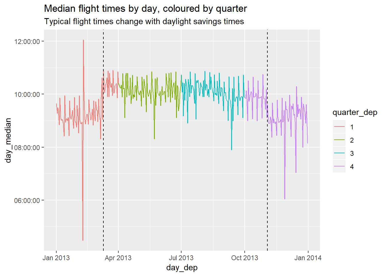

First couple and last couple months tend to have slightly earlier start times

Quantiles of flight times by month

flights_dt %>%
  transmute(month_dep = month(dep_time, label = TRUE),
            quarter_dep = quarter(dep_time) %>% factor(),
            wk_dep = week(dep_time),
            dep_time = as.hms(dep_time)) %>% 
  group_by(month_dep, wk_dep) %>% 
  ungroup() %>% 
  ggplot(aes(x = month_dep, y = dep_time, group = month_dep)) +
  geom_boxplot()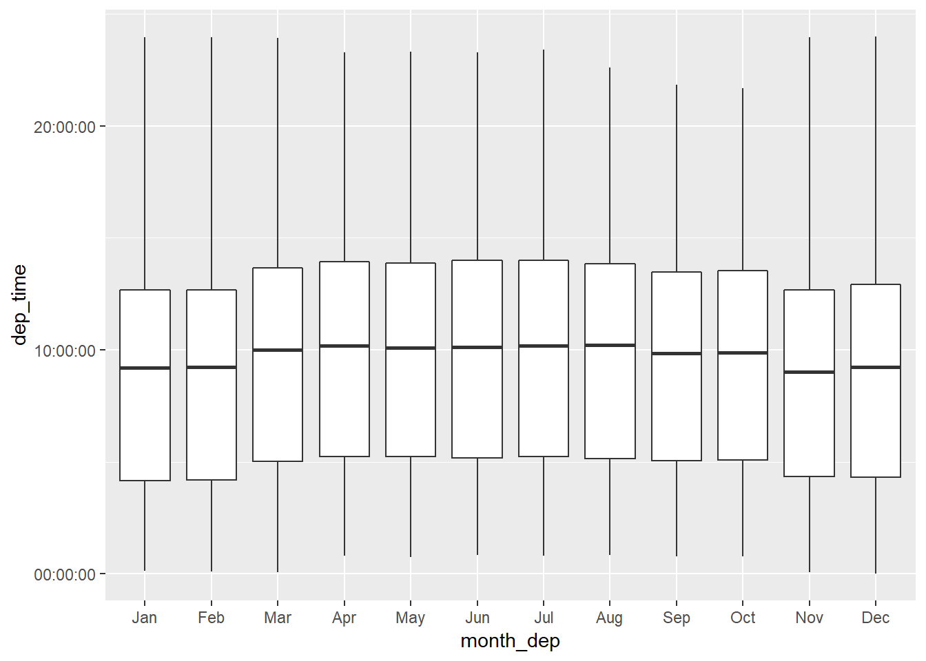

Reinforces prior plot, shows that first couple and last couple months of year tend to have slightly higher proportion of flights earlier in day
Last week of the year have a lower proportion of late flights, and a higher proportion of morning flights

See 16.3.4.1 for a few other plots I looked at.

Compare dep_time, sched_dep_time and dep_delay. Are they consistent? Explain your findings.

flights_dt %>%
  mutate(dep_delay_check = (dep_time - sched_dep_time) / dminutes(1),
         same = dep_delay == dep_delay_check,
         difference = dep_delay_check - dep_delay) %>%
  filter(abs(difference) > 0)

## # A tibble: 1,205 x 12
##    origin dest  dep_delay arr_delay dep_time            sched_dep_time     
##    <chr>  <chr>     <dbl>     <dbl> <dttm>              <dttm>             
##  1 JFK    BWI         853       851 2013-01-01 08:48:00 2013-01-01 18:35:00
##  2 JFK    SJU          43        36 2013-01-02 00:42:00 2013-01-02 23:59:00
##  3 JFK    SYR         156       154 2013-01-02 01:26:00 2013-01-02 22:50:00
##  4 JFK    SJU          33        22 2013-01-03 00:32:00 2013-01-03 23:59:00
##  5 JFK    BUF         185       172 2013-01-03 00:50:00 2013-01-03 21:45:00
##  6 JFK    BQN         156       143 2013-01-03 02:35:00 2013-01-03 23:59:00
##  7 JFK    SJU          26        23 2013-01-04 00:25:00 2013-01-04 23:59:00
##  8 JFK    PWM         141       125 2013-01-04 01:06:00 2013-01-04 22:45:00
##  9 JFK    PSE          15        18 2013-01-05 00:14:00 2013-01-05 23:59:00
## 10 JFK    FLL         127       130 2013-01-05 00:37:00 2013-01-05 22:30:00
## # ... with 1,195 more rows, and 6 more variables: arr_time <dttm>,
## #   sched_arr_time <dttm>, air_time <dbl>, dep_delay_check <dbl>,
## #   same <lgl>, difference <dbl>

They are except in the case when it goes over a day, the day is not pushed forward so it counts it as being 24 hours off

Compare air_time with the duration between the departure and arrival. Explain your findings. (Hint: consider the location of the airport.)

flights_dt %>% 
  mutate(air_time_check = (arr_time - dep_time) / dminutes(1)) %>%
  select(air_time_check, air_time, dep_time, arr_time, everything())

## # A tibble: 328,063 x 10
##    air_time_check air_time dep_time            arr_time            origin
##             <dbl>    <dbl> <dttm>              <dttm>              <chr> 
##  1            193      227 2013-01-01 05:17:00 2013-01-01 08:30:00 EWR   
##  2            197      227 2013-01-01 05:33:00 2013-01-01 08:50:00 LGA   
##  3            221      160 2013-01-01 05:42:00 2013-01-01 09:23:00 JFK   
##  4            260      183 2013-01-01 05:44:00 2013-01-01 10:04:00 JFK   
##  5            138      116 2013-01-01 05:54:00 2013-01-01 08:12:00 LGA   
##  6            106      150 2013-01-01 05:54:00 2013-01-01 07:40:00 EWR   
##  7            198      158 2013-01-01 05:55:00 2013-01-01 09:13:00 EWR   
##  8             72       53 2013-01-01 05:57:00 2013-01-01 07:09:00 LGA   
##  9            161      140 2013-01-01 05:57:00 2013-01-01 08:38:00 JFK   
## 10            115      138 2013-01-01 05:58:00 2013-01-01 07:53:00 LGA   
## # ... with 328,053 more rows, and 5 more variables: dest <chr>,
## #   dep_delay <dbl>, arr_delay <dbl>, sched_dep_time <dttm>,
## #   sched_arr_time <dttm>

Initial check is off, so need to take into account the time-zone and difference from NYC, so join timezone document

flights_dt %>% 
  left_join(select(nycflights13::airports, dest = faa, tz), by = "dest") %>% 
  mutate(arr_time_new = arr_time - dhours(tz + 5)) %>% 
  mutate(air_time_tz = (arr_time_new - dep_time) / dminutes(1),
         diff_Airtime = air_time_tz - air_time) %>% 
  select( origin, dest, tz, contains("time"), -(contains("sched")))

## # A tibble: 328,063 x 9
##    origin dest     tz dep_time            arr_time            air_time
##    <chr>  <chr> <dbl> <dttm>              <dttm>                 <dbl>
##  1 EWR    IAH      -6 2013-01-01 05:17:00 2013-01-01 08:30:00      227
##  2 LGA    IAH      -6 2013-01-01 05:33:00 2013-01-01 08:50:00      227
##  3 JFK    MIA      -5 2013-01-01 05:42:00 2013-01-01 09:23:00      160
##  4 JFK    BQN      NA 2013-01-01 05:44:00 2013-01-01 10:04:00      183
##  5 LGA    ATL      -5 2013-01-01 05:54:00 2013-01-01 08:12:00      116
##  6 EWR    ORD      -6 2013-01-01 05:54:00 2013-01-01 07:40:00      150
##  7 EWR    FLL      -5 2013-01-01 05:55:00 2013-01-01 09:13:00      158
##  8 LGA    IAD      -5 2013-01-01 05:57:00 2013-01-01 07:09:00       53
##  9 JFK    MCO      -5 2013-01-01 05:57:00 2013-01-01 08:38:00      140
## 10 LGA    ORD      -6 2013-01-01 05:58:00 2013-01-01 07:53:00      138
## # ... with 328,053 more rows, and 3 more variables: arr_time_new <dttm>,
## #   air_time_tz <dbl>, diff_Airtime <dbl>

Is closer but still off. In chapter 5, problem 5.5.2.1 I go further into this
In Appendix section 16.3.4.3 filter to NAs

How does the average delay time change over the course of a day? Should you use dep_time or sched_dep_time? Why?

flights_dt %>% 
  mutate(sched_dep_time = as.hms(floor_date(sched_dep_time, "30 mins"))) %>%
  group_by(sched_dep_time) %>%
  summarise(delay_mean = mean(arr_delay, na.rm = TRUE), 
            n = n(),
            n_na = sum(is.na(arr_delay)) / n,
            delay_median = median(arr_delay, na.rm = TRUE)) %>% 
  ggplot(aes(x = sched_dep_time, y = delay_mean, size = n)) +
  geom_point()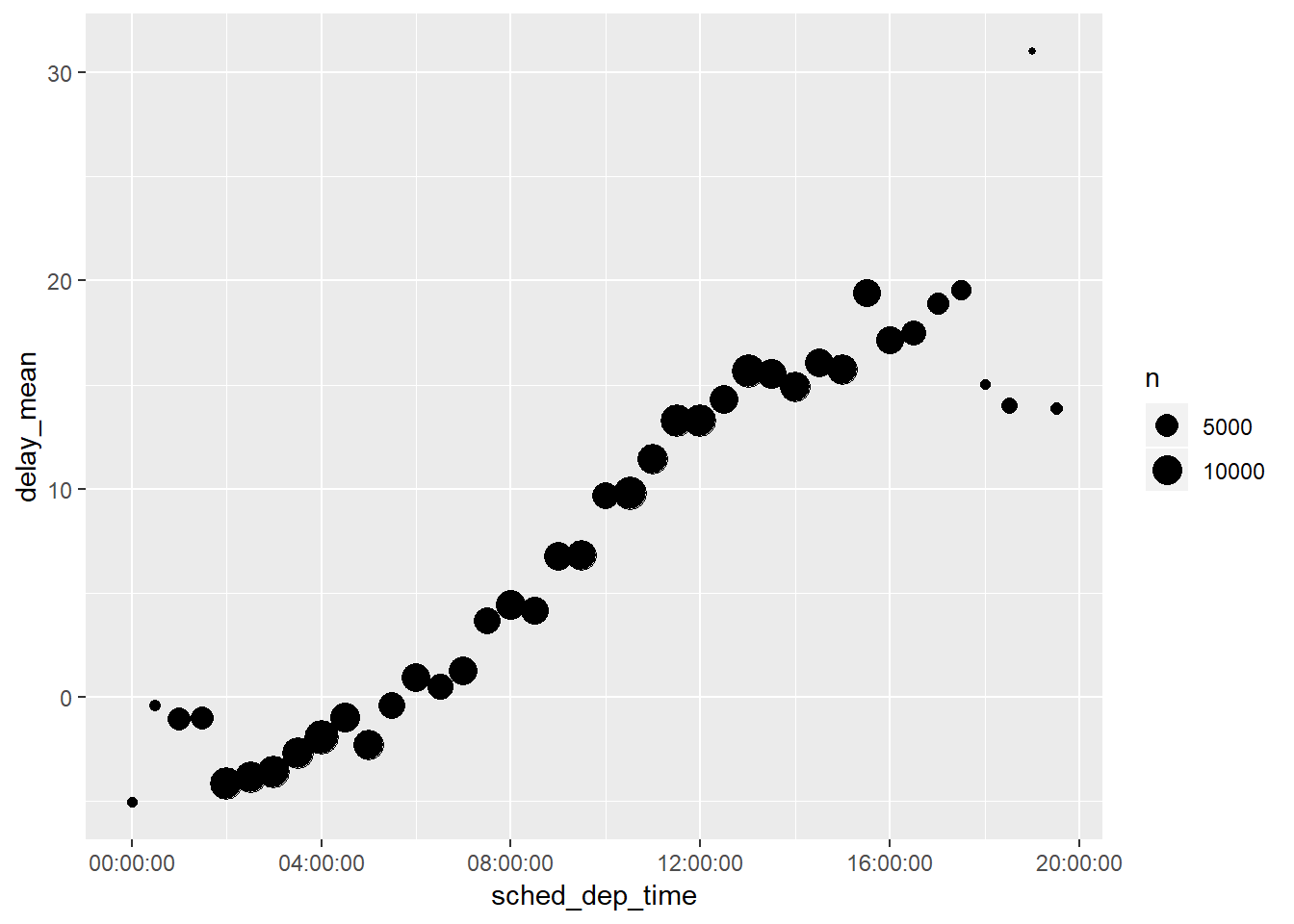

It goes-up throughout the day
Use sched_dep_time because it has the correct day

On what day of the week should you leave if you want to minimise the chance of a delay?

flights_dt %>%
  mutate(weekday = wday(sched_dep_time, label = TRUE)) %>%
  group_by(weekday) %>%
  summarise(prop_delay = sum(dep_delay > 0) / n())

## # A tibble: 7 x 2
##   weekday prop_delay
##   <ord>        <dbl>
## 1 Sun          0.383
## 2 Mon          0.401
## 3 Tue          0.364
## 4 Wed          0.372
## 5 Thu          0.431
## 6 Fri          0.425
## 7 Sat          0.348

wknd has a slightly lower proportion of flights delayed (Thursday has the worst)

What makes the distribution of diamonds$carat and flights$sched_dep_time similar?

ggplot(diamonds, aes(x = carat)) +
  geom_histogram(bins = 500)+
  labs(title = "Distribution of carat in diamonds dataset")

ggplot(flights, aes(x = as.hms(sched_dep_time))) +
  geom_histogram(bins = 24*6)+
  labs(title = "Distribution of scheduled departure times in flights dataset")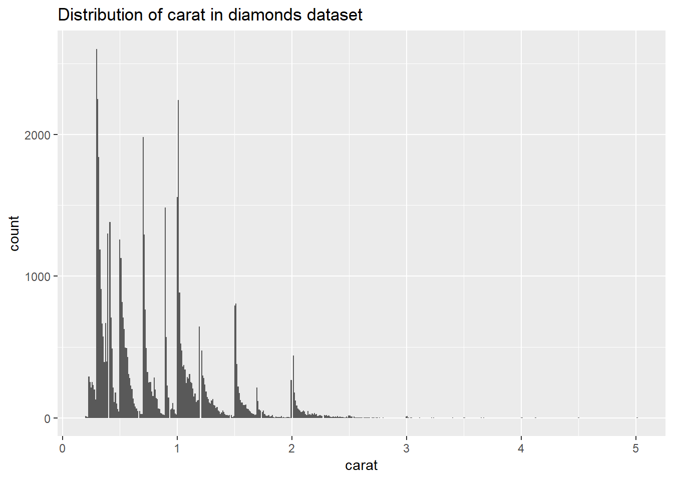

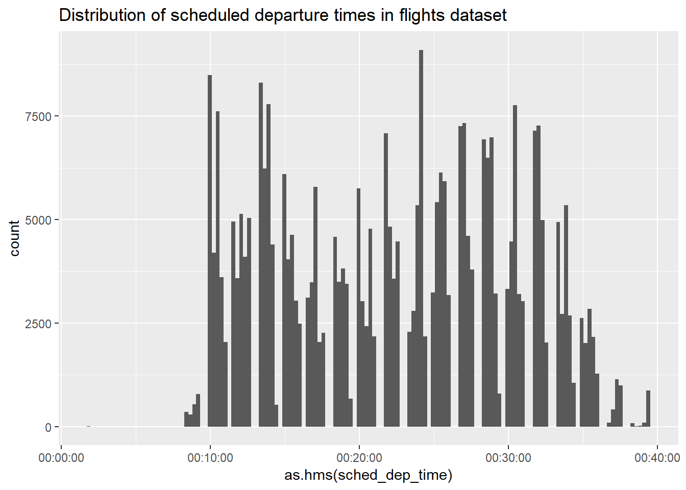
Both have gaps and peaks at ‘attractive’ values

Confirm my hypothesis that the early departures of flights in minutes 20-30 and 50-60 are caused by scheduled flights that leave early. Hint: create a binary variable that tells you whether or not a flight was delayed.

mutate(flights_dt,
       mins_dep = minute(dep_time),
       mins_sched = minute(sched_dep_time),
       delayed = dep_delay > 0) %>%
  group_by(mins_dep) %>%
  summarise(prop_delayed = sum(delayed) / n()) %>%
  ggplot(aes(x = mins_dep, y = prop_delayed)) +
  geom_line()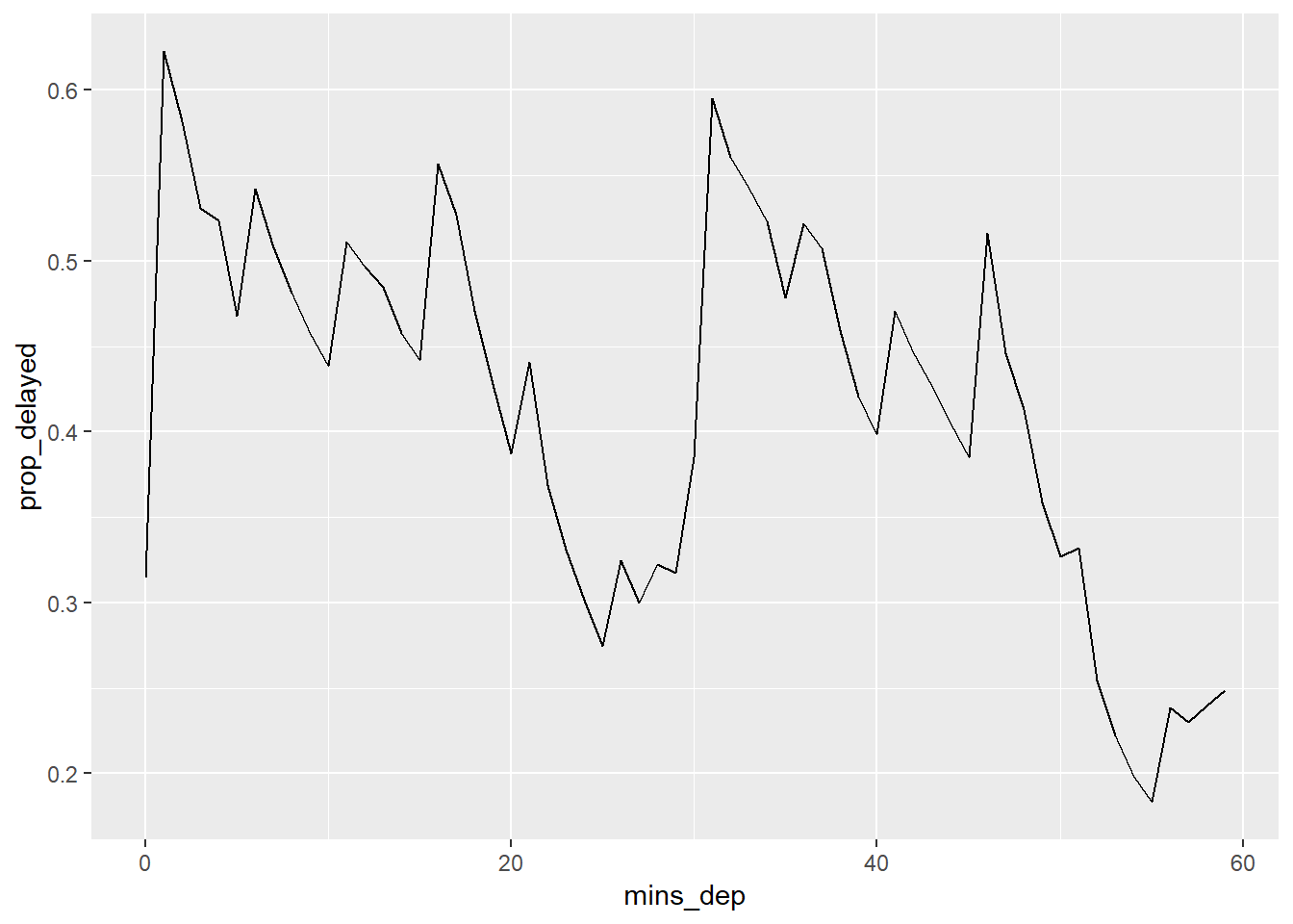

Consistent with above hypothesis

16.4: Time spans

durations, which represent an exact number of seconds.
periods, which represent human units like weeks and months.
intervals, which represent a starting and ending point.

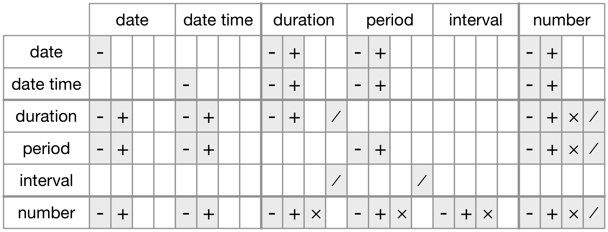
Permitted arithmetic operations between different data types

Periods example, using durations to fix oddity of problem when flight arrives overnight

flights_dt <- flights_dt %>% 
  mutate(
    overnight = arr_time < dep_time,
    arr_time = arr_time + days(overnight * 1),
    sched_arr_time = sched_arr_time + days(overnight * 1)
  )

Intervals example to get precise number of days dependent on specific time

next_year <- today() + years(1)
(today() %--% next_year) / ddays(1)

## [1] 366

To find out how many periods fall in an interval, need to use integer division

(today() %--% next_year) %/% days(1)

## Note: method with signature 'Timespan#Timespan' chosen for function '%/%',
##  target signature 'Interval#Period'.
##  "Interval#ANY", "ANY#Period" would also be valid

## [1] 366

16.4.5

Why is there months() but no dmonths()?
- the duration varies from month to month
Explain days(overnight * 1) to someone who has just started learning R. How does it work?
- this used in the example above makes it such that if overnight is TRUE, it will return the same time period but one day ahead, if false, does not change (as is adding 0 days)

Create a vector of dates giving the first day of every month in 2015.

x <- ymd("2015-01-01")
mons <- c(0:11)
(x + months(mons)) %>% wday(label = TRUE)

##  [1] Thu Sun Sun Wed Fri Mon Wed Sat Tue Thu Sun Tue
## Levels: Sun < Mon < Tue < Wed < Thu < Fri < Sat

Create a vector of dates giving the first day of every month in the current year.

x <- today() %>% update(month = 1, mday = 1)
mons <- c(0:11)
(x + months(mons)) %>% wday(label=TRUE)

##  [1] Tue Fri Fri Mon Wed Sat Mon Thu Sun Tue Fri Sun
## Levels: Sun < Mon < Tue < Wed < Thu < Fri < Sat

Write a function that given your birthday (as a date), returns how old you are in years.

birthday_age <- function(birthday) {
  (ymd(birthday) %--% today()) %/% years(1)
}
birthday_age("1989-09-07")

## [1] 29

Why can’t (today() %--% (today() + years(1)) / months(1) work?
- Can’t add and subtract intervals

Appendix

16.3.4.1

Weekly flight proportions by 4 hour blocks

flights_dt %>%
  transmute(month_dep = month(dep_time, label = TRUE),
            wk_dep = week(dep_time),
            dep_time_4hrs = floor_date(dep_time, "4 hours"),
            hour_dep_4hrs = hour(dep_time_4hrs) %>% factor) %>% 
  count(wk_dep, hour_dep_4hrs) %>%
  group_by(wk_dep) %>% 
  mutate(wk_tot = sum(n), 
         wk_prop = round(n / wk_tot, 3)) %>% 
  ungroup() %>% 
  ggplot(aes(x = wk_dep, y = wk_prop)) +
  geom_col(aes(fill = hour_dep_4hrs))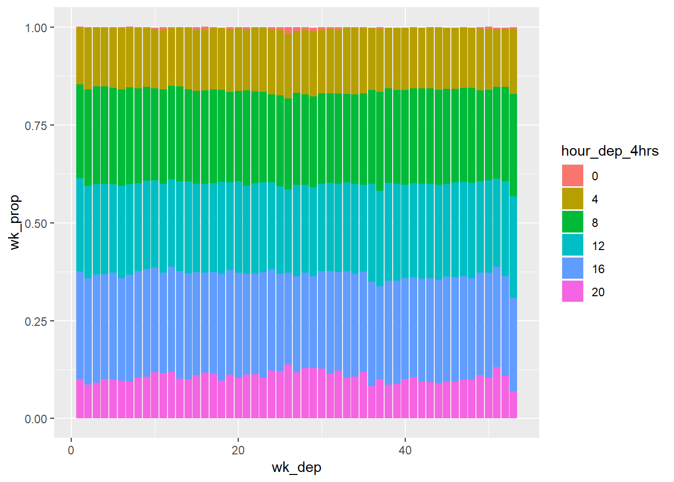

Weekly median fight time

flights_dt %>%
  transmute(quarter_dep = quarter(dep_time) %>% factor(),
            day_dep = as_date(dep_time),
            wk_dep = floor_date(dep_time, "1 week") %>% as_date,
            dep_time = as.hms(dep_time)) %>% 
  group_by(quarter_dep, wk_dep) %>% 
  summarise(wk_median = median(dep_time)) %>% 
  ungroup() %>% 
  mutate(wk_median = as.hms(wk_median)) %>% 
  ggplot(aes(x = wk_dep, y = wk_median)) +
  geom_line(aes(colour = quarter_dep, group = 1))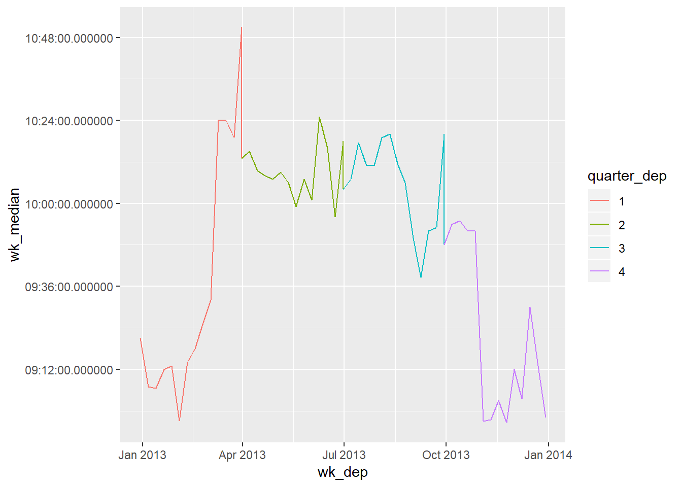

Proportion of flights in each hour, by quarter

flights_dt %>%
  transmute(quarter_dep = quarter(dep_time) %>% factor(),
            hour_dep = hour(dep_time)) %>% 
  count(quarter_dep, hour_dep) %>%
  group_by(quarter_dep) %>% 
  mutate(quarter_tot = sum(n), 
         quarter_prop = round(n / quarter_tot, 3)) %>% 
  ungroup() %>% 
    ggplot(aes(x = hour_dep, y = quarter_prop)) +
    geom_line(aes(colour = quarter_dep))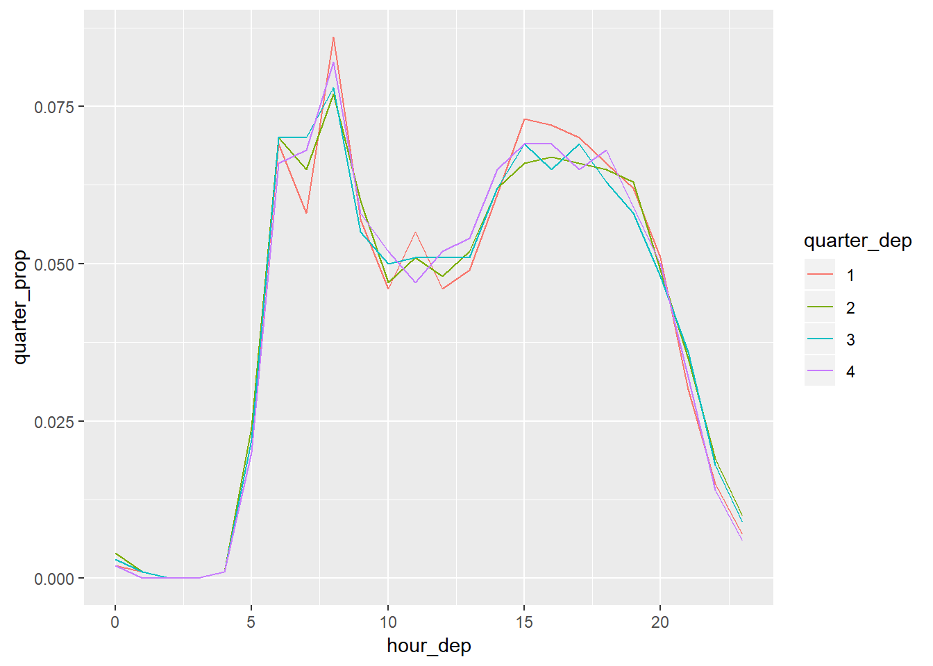

Q1 seems to be a little more extreme at the local maximas

Look at proportion of flights by hour faceted by each month

flights_dt %>%
  transmute(month_dep = month(dep_time, label = TRUE),
            hour_dep = hour(dep_time)) %>% 
  count(month_dep, hour_dep) %>%
  group_by(month_dep) %>% 
  mutate(month_tot = sum(n), 
         month_prop = round(n / month_tot, 3)) %>% 
  ungroup() %>% 
  ggplot(aes(x = hour_dep, y = month_prop)) +
  geom_line() +
  facet_wrap( ~ month_dep)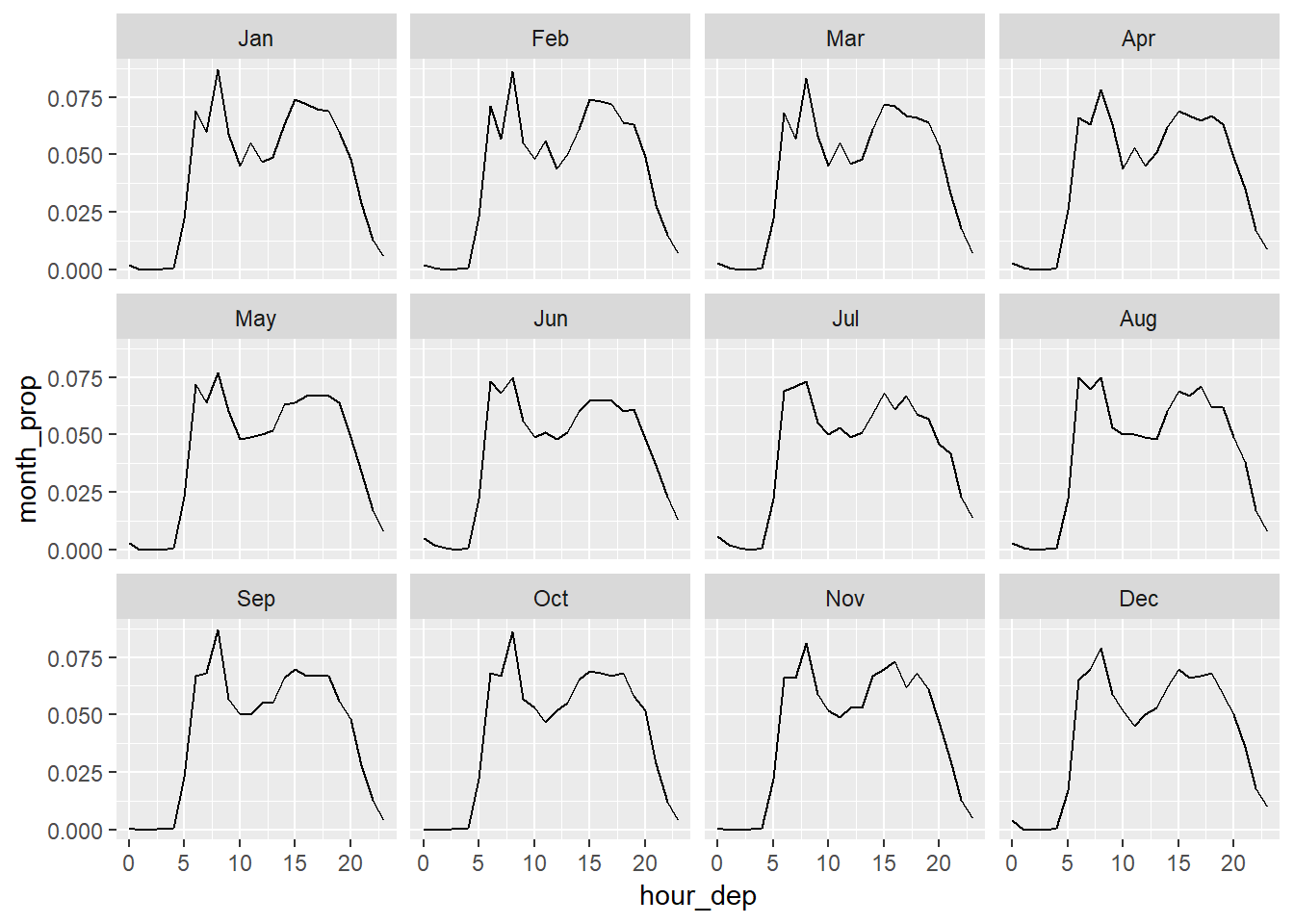

16.3.4.3

Perhaps these are flights where landed in different location…

flights_dt %>% 
  mutate(arr_delay_test = (arr_time - sched_arr_time) / dminutes(1)) %>% 
  select( origin, dest, dep_delay, arr_delay, arr_delay_test, contains("time")) %>% 
  filter(is.na(arr_delay))

## # A tibble: 717 x 10
##    origin dest  dep_delay arr_delay arr_delay_test dep_time           
##    <chr>  <chr>     <dbl>     <dbl>          <dbl> <dttm>             
##  1 LGA    XNA          -5        NA             89 2013-01-01 15:25:00
##  2 EWR    STL          29        NA            195 2013-01-01 15:28:00
##  3 LGA    XNA          -5        NA             98 2013-01-01 17:40:00
##  4 EWR    SAN          29        NA            108 2013-01-01 18:07:00
##  5 JFK    DFW          59        NA          -1282 2013-01-01 19:39:00
##  6 EWR    TUL          22        NA            111 2013-01-01 19:52:00
##  7 EWR    XNA          43        NA            148 2013-01-02 09:05:00
##  8 LGA    GRR         120        NA            179 2013-01-02 11:25:00
##  9 JFK    DFW           8        NA            102 2013-01-02 18:48:00
## 10 EWR    MCI          85        NA            177 2013-01-02 18:49:00
## # ... with 707 more rows, and 4 more variables: sched_dep_time <dttm>,
## #   arr_time <dttm>, sched_arr_time <dttm>, air_time <dbl>

16.3.4.4

Below started looking at proportions…

mutate(flights_dt,
       dep_old = dep_time,
       sched_old = sched_dep_time,
       dep_time = floor_date(dep_time, "5 minutes"),
       sched_dep_time = floor_date(sched_dep_time, "5 minutes"),
       mins_dep = minute(dep_time),
       mins_sched = minute(sched_dep_time),
       delayed = dep_delay > 0) %>%
  group_by(mins_dep, mins_sched) %>%
  summarise(num_delayed = sum(delayed),
            num = n(),
            prop_delayed = num_delayed / num) %>% 
  group_by(mins_dep) %>% 
  mutate(num_tot = sum(num),
         prop_sched = num / num_tot,
         sched_dep_diff = mins_dep - mins_sched) %>% 
  ungroup() %>% 
  ggplot(aes(x = mins_dep, y = prop_sched, fill = factor(mins_sched))) +
  geom_col()+
  labs(title = "Proportion of early flights by minute scheduled v. minute departed")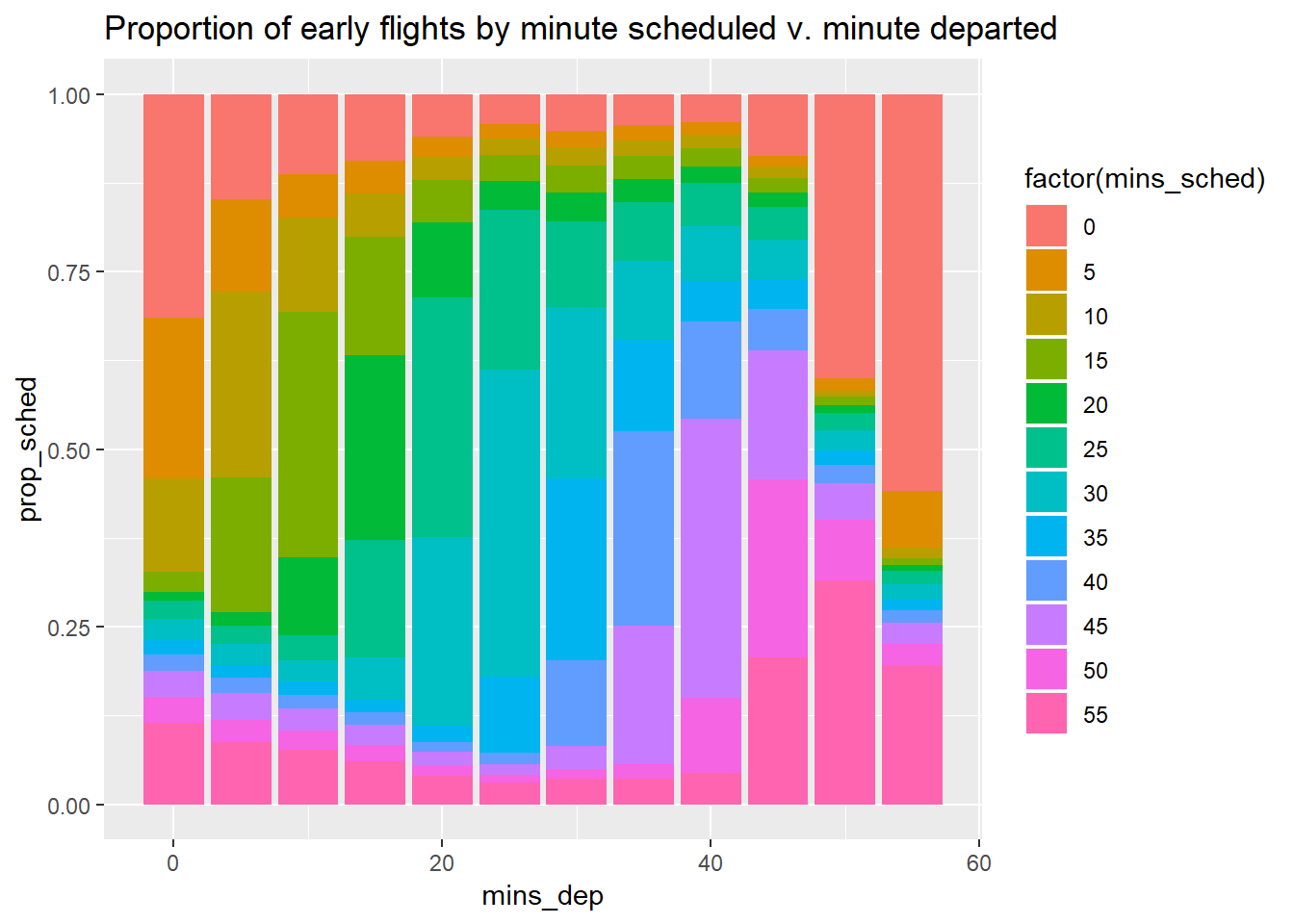

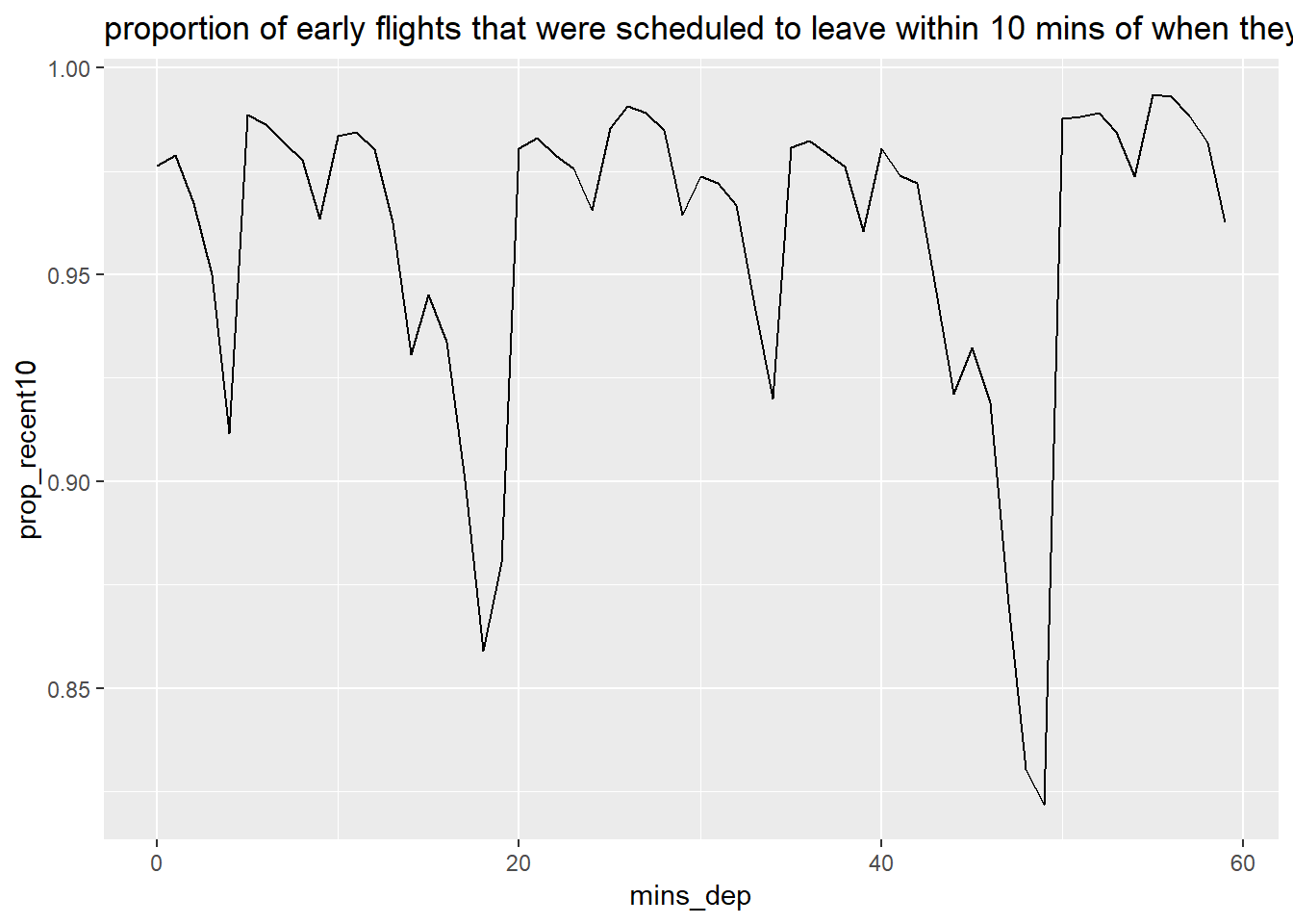
  mutate(flights_dt,
       dep_old = dep_time,
       sched_old = sched_dep_time,
       # dep_time = floor_date(dep_time, "5 minutes"),
       # sched_dep_time = floor_date(sched_dep_time, "5 minutes"),
       mins_dep = minute(dep_time),
       mins_sched = minute(sched_dep_time),
       early_less10 = dep_delay >= -10) %>%
  filter(dep_delay < 0) %>% 
  group_by(mins_dep) %>%
  summarise(num = n(),
            sum_recent10 = sum(early_less10),
            prop_recent10 = sum_recent10 / num) %>% 
  ungroup() %>% 
  ggplot(aes(x = mins_dep, y = prop_recent10)) +
  geom_line()+
  labs(title = "proportion of early flights that were scheduled to leave within 10 mins of when they did")