Ch. 21: Iteration
Key questions:
- 21.2.1. #1, 2
- 21.3.5. #1, 3
- 21.4.1. #2
- 21.5.3. #1
- 21.9.4. #2
- Common
forloop template:
output <- vector("double", ncol(df)) # common for loop style
for (i in seq_len(length(df))){
  output[[i]] <- fun(df[[i]])
} - Common
whileloop template:
i <- 1
while (i <= length(x)){
  # body
  i <- i + 1
} seq_along(df)does essentially same asseq_len(length(df))unlistflatten list of vectors into single vectorflaten_dblis stricter alternative
dplyr::bind_rowssave output in a list of dfs and then append all at end rather than sequentialrbindingsample(c("T", "H"), 1)sapplyis wrapper aroundlapplythat automatically simplifies output – problematic in that never know what ouptut will bevapplyis safe alternative tosapplye.g. for logicalvapply(df, is.numeric, logical(1)), butmap_lgl(df, is.numeric)is more simplemap()makes a list.map_lgl()makes a logical vector.map_int()makes an integer vector.map_dbl()makes a double vector.map_chr()makes a character vector.
- shortcuts for applying functions in
map:
models <- mtcars %>%
  split(.$cyl) %>%
  map(function(df) lm(mpg ~ wt, data = df))

models <- mtcars %>%
  split(.$cyl) %>%
map(~lm(mpg ~ wt, data = .))- extracting by named elements from
map:
models %>%
  map(summary) %>%
map_dbl("r.squared")- extracting by positions from
map
x <- list(list(1, 2, 3), list(4, 5, 6), list(7, 8, 9))
x %>%
map_dbl(2)map2let’s you iterate through two components at oncepmapallows you to iterate over p components – works well to hold inputs in a dataframesafelytakes funciton returns two parts, result and error object- similar to
trybut more consistent
- similar to
possiblysimilar to safely, but provide it a default value to return for errorsquietlyis similar to safely but captures all printed output messages and warningspurrr::transposeallows you to do things like get all 2nd elements in list, e.g. show laterinvoke_maplet’s you iterate over both the functions and the parameters, have anfand aparaminput, e.g.
f <- c("runif", "rnorm", "rpois")
param <- list(
  list(min = -1, max = 1),
  list(sd = 5),
  list(lambda = 10)
)

invoke_map(f, param, n = 5) %>% str()walkis alternative tomapthat you call for side effects. Also havewalk2andpwalkthat are generally more useful- all invisibly return `.x (the first argument) so can used in the middle of pipelines
keepanddiscardkeep or discard elements in the input based off ifTRUEto predicatesomeandeverydetermine if the predicte is true for any or for all of our elementsdetectfinds the first element where the predicate is true,detect_indexreturns its positionhead_whileandtail_whiletake elements from the start or end of a vector while a predicate is truereduceis good for applying two table rule repeatedly, e.g. joinsaccumulateis similar but keeps all the interim results
21.2: For loops
21.2.1
Write for loops to (think about the output, sequence, and body before you start writing the loop):
- Compute the mean of every column in
mtcars.
output <- vector("double", length(mtcars))
for (i in seq_along(mtcars)){
  output[[i]] <- mean(mtcars[[i]])
}
output
## [1] 20.090625 6.187500 230.721875 146.687500 3.596563 3.217250 ## [7] 17.848750 0.437500 0.406250 3.687500 2.812500- Determine the type of each column in
nycflights13::flights.
output <- vector("character", length(flights))
for (i in seq_along(flights)){
  output[[i]] <- typeof(flights[[i]])
}
output
## [1] "integer" "integer" "integer" "integer" "integer" ## [6] "double" "integer" "integer" "double" "character" ## [11] "integer" "character" "character" "character" "double" ## [16] "double" "double" "double" "double"- Compute the number of unique values in each column of
iris.
output <- vector("integer", length(iris))
for (i in seq_along(iris)){
  output[[i]] <- unique(iris[[i]]) %>% length()
}
output
## [1] 35 23 43 22 3- Generate 10 random normals for each of \(\mu = -10\), \(0\), \(10\), and \(100\).
output <- vector("list", 4)
input_means <- c(-10, 0, 10, 100)
for (i in seq_along(output)){
  output[[i]] <- rnorm(10, mean = input_means[[i]])
}
output
## [[1]] ## [1] -11.371326 -10.118467 -10.582961 -10.324829 -7.604983 -9.300232 ## [7] -9.840124 -9.719733 -9.784274 -10.338814 ## ## [[2]] ## [1] -1.04951842 -0.68385670 0.17893523 0.07338463 -1.18028235 ## [6] -1.00777188 0.91491408 -0.14041984 -0.25074297 -0.50055019 ## ## [[3]] ## [1] 11.013913 9.790495 10.631115 10.325991 10.608040 9.463515 11.265961 ## [8] 10.630382 10.436201 8.907654 ## ## [[4]] ## [1] 99.37012 100.31396 99.06230 98.00350 100.31506 99.67347 101.02248 ## [8] 98.32484 98.62669 100.28487- Compute the mean of every column in
Eliminate the for loop in each of the following examples by taking advantage of an existing function that works with vectors:
example:
out <- "" for (x in letters) { out <- stringr::str_c(out, x) } out- collabse letters into length-one character vector with all characters concatenated
str_c(letters, collapse = "")## [1] "abcdefghijklmnopqrstuvwxyz"example:
x <- sample(100)
sd <- 0
for (i in seq_along(x)) {
  sd <- sd + (x[i] - mean(x)) ^ 2
}
sd <- sqrt(sd / (length(x) - 1))
sd
## [1] 29.01149- calculate standard deviaiton of x
sd(x)## [1] 29.01149example:
x <- runif(100)
out <- vector("numeric", length(x))
out[1] <- x[1]
for (i in 2:length(x)) {
  out[i] <- out[i - 1] + x[i]
}
out
## [1] 0.1543797 0.5168570 1.4323513 1.4861995 1.7440626 2.3503876 ## [7] 2.7033856 3.4933038 3.8878801 4.8166162 4.8404351 5.0134399 ## [13] 5.8128633 5.9002886 6.4672338 7.3249551 7.4813311 7.9067374 ## [19] 7.9143362 8.6500421 9.4114592 9.8109883 10.6637337 11.5345437 ## [25] 11.8881403 12.8609933 13.0060893 13.1121490 13.2820768 13.7832678 ## [31] 14.0103818 14.8921300 15.8878166 16.3724888 17.2897726 17.6764167 ## [37] 18.3759822 18.5914902 18.7581008 19.3126850 20.0314901 20.9729033 ## [43] 21.5123325 22.1361972 22.9338153 23.9220106 23.9905409 24.1247463 ## [49] 24.3690186 24.6778073 25.1676470 25.6649358 26.0152919 26.3936317 ## [55] 26.6769802 26.7589431 27.4933689 28.3744835 28.8274173 29.5040112 ## [61] 30.4625068 31.1908181 31.5785996 32.0691594 32.4015008 33.1859971 ## [67] 34.0973779 34.4118215 34.6828655 34.9383821 35.5988994 35.9820211 ## [73] 36.7825814 37.5402040 37.9568733 38.5686788 38.6336509 39.0451422 ## [79] 39.1208101 39.8826954 40.4989736 41.2877620 41.4204198 41.8790701 ## [85] 42.8085235 43.2102977 43.4620636 43.9427926 44.7306195 45.4886119 ## [91] 46.0891834 46.4679661 47.0817039 47.6331389 48.1357901 48.3671822 ## [97] 48.8290107 49.8198761 50.6520274 50.6527903- calculate cumulative sum
cumsum(x)## [1] 0.1543797 0.5168570 1.4323513 1.4861995 1.7440626 2.3503876 ## [7] 2.7033856 3.4933038 3.8878801 4.8166162 4.8404351 5.0134399 ## [13] 5.8128633 5.9002886 6.4672338 7.3249551 7.4813311 7.9067374 ## [19] 7.9143362 8.6500421 9.4114592 9.8109883 10.6637337 11.5345437 ## [25] 11.8881403 12.8609933 13.0060893 13.1121490 13.2820768 13.7832678 ## [31] 14.0103818 14.8921300 15.8878166 16.3724888 17.2897726 17.6764167 ## [37] 18.3759822 18.5914902 18.7581008 19.3126850 20.0314901 20.9729033 ## [43] 21.5123325 22.1361972 22.9338153 23.9220106 23.9905409 24.1247463 ## [49] 24.3690186 24.6778073 25.1676470 25.6649358 26.0152919 26.3936317 ## [55] 26.6769802 26.7589431 27.4933689 28.3744835 28.8274173 29.5040112 ## [61] 30.4625068 31.1908181 31.5785996 32.0691594 32.4015008 33.1859971 ## [67] 34.0973779 34.4118215 34.6828655 34.9383821 35.5988994 35.9820211 ## [73] 36.7825814 37.5402040 37.9568733 38.5686788 38.6336509 39.0451422 ## [79] 39.1208101 39.8826954 40.4989736 41.2877620 41.4204198 41.8790701 ## [85] 42.8085235 43.2102977 43.4620636 43.9427926 44.7306195 45.4886119 ## [91] 46.0891834 46.4679661 47.0817039 47.6331389 48.1357901 48.3671822 ## [97] 48.8290107 49.8198761 50.6520274 50.6527903Combine your function writing and for loop skills:
- Write a for loop that
prints()the lyrics to the children’s song “Alice the camel”.
num_humps <- c("five", "four", "three", "two", "one", "no")

for (i in seq_along(num_humps)){

  paste0("Alice the camel has ", num_humps[[i]], " humps.") %>%
    rep(3) %>%
    writeLines()

  writeLines("So go, Alice, go.\n")
}
## Alice the camel has five humps. ## Alice the camel has five humps. ## Alice the camel has five humps. ## So go, Alice, go. ## ## Alice the camel has four humps. ## Alice the camel has four humps. ## Alice the camel has four humps. ## So go, Alice, go. ## ## Alice the camel has three humps. ## Alice the camel has three humps. ## Alice the camel has three humps. ## So go, Alice, go. ## ## Alice the camel has two humps. ## Alice the camel has two humps. ## Alice the camel has two humps. ## So go, Alice, go. ## ## Alice the camel has one humps. ## Alice the camel has one humps. ## Alice the camel has one humps. ## So go, Alice, go. ## ## Alice the camel has no humps. ## Alice the camel has no humps. ## Alice the camel has no humps. ## So go, Alice, go.- Convert the nursery rhyme “ten in the bed” to a function. Generalise it to any number of people in any sleeping structure.
nursery_bed <- function(num, y) {
  output <- vector("character", num)
  for (i in seq_along(output)) {
    output[[i]] <- str_replace_all(
    'There were x in the _y\n And the little one said, \n"Roll over! Roll over!"\n So they all rolled over and\n one fell out.', c("x" = (length(output) - i + 1), "_y" = y))
  }
  str_c(output, collapse = "\n\n") %>%
    writeLines()
}

nursery_bed(3, "asteroid")
## There were 3 in the asteroid ## And the little one said, ## "Roll over! Roll over!" ## So they all rolled over and ## one fell out. ## ## There were 2 in the asteroid ## And the little one said, ## "Roll over! Roll over!" ## So they all rolled over and ## one fell out. ## ## There were 1 in the asteroid ## And the little one said, ## "Roll over! Roll over!" ## So they all rolled over and ## one fell out.- Convert the song “99 bottles of beer on the wall” to a function. Generalise to any number of any vessel containing any liquid on any surface.
- This is a little bit of a lazy version…
beer_rhyme <- function(x, y, z){
  output <- vector("character", x)
  for (i in seq_along(output)){
    output[i] <-
      str_replace_all("x bottles of y on the z.\n One fell off...", c(
      "x" = (x - i + 1),
      "y" = y,
      "z" = z
      ))
  }
  output <- (str_c(output, collapse = "\n") %>%
               str_c("\nNo more bottles...", collapse = ""))
  writeLines(output)
}

beer_rhyme(4, "soda", "toilet")
## 4 bottles of soda on the toilet. ## One fell off... ## 3 bottles of soda on the toilet. ## One fell off... ## 2 bottles of soda on the toilet. ## One fell off... ## 1 bottles of soda on the toilet. ## One fell off... ## No more bottles...- Write a for loop that
It’s common to see for loops that don’t preallocate the output and instead increase the length of a vector at each step. How does this affect performance? Design and execute an experiment.
preallocate <- function(){
x <- vector("double", 100)
  for (i in seq_along(x)){
    x[i] <- rnorm(1)
  }
}

growing <- function(){
  x <- c(0)
    for (i in 1:100){
      x[i] <- rnorm(1)
  }
}

microbenchmark::microbenchmark(
  space = preallocate(),
  no_space = growing(),
  times = 20
)
## Unit: microseconds ## expr min lq mean median uq max neval cld ## space 178.0 183.6 523.665 308.05 342.65 4991.2 20 a ## no_space 213.6 222.2 531.440 344.50 429.05 4081.9 20 a- see roughly 35% better performance when creating ahead of time
- note: if you can do these operations with vectorized approach though – they’re often much faster
microbenchmark::microbenchmark(
  space = preallocate(),
  no_space = growing(),
  vector = rnorm(100),
  times = 20
)
## Unit: microseconds ## expr min lq mean median uq max neval cld ## space 155.8 161.45 177.075 163.50 166.20 349.6 20 b ## no_space 185.8 193.65 202.390 199.55 205.25 234.5 20 c ## vector 8.8 9.45 9.795 9.70 10.10 11.0 20 a- vectorized was > 10x faster
21.3 For loop variations
21.3.5
Imagine you have a directory full of CSV files that you want to read in. You have their paths in a vector,
files <- dir("data/", pattern = "\\.csv$", full.names = TRUE), and now want to read each one withread_csv(). Write the for loop that will load them into a single data frame.- To start this problem, I first created a file directory, and then wrote in 26 csvs each with the most popular name from each year since 1880 for a particular letter35.
- Next I read these into a single dataframe with a for loop
What happens if you use
for (nm in names(x))andxhas no names?x <- list(1:10, 11:18, 19:25) for (nm in names(x)) { print(x[[nm]]) }- each iteration produces an error, so nothing is written
What if only some of the elements are named?
x <- list(a = 1:10, 11:18, c = 19:25)
for (nm in names(x)) {
  print(x[[nm]])
}
## [1] 1 2 3 4 5 6 7 8 9 10 ## NULL ## [1] 19 20 21 22 23 24 25- you have output for those with names and NULL for those without
What if the names are not unique?
x <- list(a = 1:10, a = 11:18, c = 19:25)
for (nm in names(x)) {
  print(x[[nm]])
}
## [1] 1 2 3 4 5 6 7 8 9 10 ## [1] 1 2 3 4 5 6 7 8 9 10 ## [1] 19 20 21 22 23 24 25- it prints the first position with the name
Write a function that prints the mean of each numeric column in a data frame, along with its name. For example,
show_mean(iris)would print:show_mean(iris) #> Sepal.Length: 5.84 #> Sepal.Width: 3.06 #> Petal.Length: 3.76 #> Petal.Width: 1.20(Extra challenge: what function did I use to make sure that the numbers lined up nicely, even though the variable names had different lengths?)
show_mean <- function(df){
  # select just cols that are numeric
  out <- vector("logical", length(df))
  for (i in seq_along(df)) {
    out[[i]] <- is.numeric(df[[i]])
  }
  df_select <- df[out]
  # keep/discard funs would have made this easy

  # make list of values w/ mean
  means <- vector("list", length(df_select))
  names(means) <- names(df_select)
  for (i in seq_along(df_select)){
    means[[i]] <- mean(df_select[[i]], na.rm = TRUE) %>%
      round(digits = 2)
  }

  # print out, use method to identify max chars for vars printed
  means_names <- names(means)
  chars_max <- (str_count(means_names) + str_count(as.character(means))) %>%
    max()

  chars_pad <- chars_max - (str_count(means_names) + str_count(as.character(means)))

  names(chars_pad) <- means_names

str_c(means_names, ": ", str_dup(" ", chars_pad), means) %>%
  writeLines()
}

show_mean(flights)
## year: 2013 ## month: 6.55 ## day: 15.71 ## dep_time: 1349.11 ## sched_dep_time: 1344.25 ## dep_delay: 12.64 ## arr_time: 1502.05 ## sched_arr_time: 1536.38 ## arr_delay: 6.9 ## flight: 1971.92 ## air_time: 150.69 ## distance: 1039.91 ## hour: 13.18 ## minute: 26.23What does this code do? How does it work?
trans <- list( disp = function(x) x * 0.0163871, am = function(x) { factor(x, labels = c("auto", "manual")) } ) for (var in names(trans)) { mtcars[[var]] <- trans[[var]](mtcars[[var]]) } mtcars- first part builds list of functions, 2nd applies those to a dataset
- are storing the data transformations as a function and then applying this to a dataframe36
21.4: For loops vs. functionals
21.4.1
Read the documentation for
apply(). In the 2d case, what two for loops does it generalise?- It allows you to input either 1 or 2 for the
MARGINargument, which corresponds with looping over either the rows or the columns.
- It allows you to input either 1 or 2 for the
Adapt
col_summary()so that it only applies to numeric columns You might want to start with anis_numeric()function that returns a logical vector that has a TRUE corresponding to each numeric column.col_summary_gen <- function(df, fun, ...) { #find cols that are numeric out <- vector("logical", length(df)) for (i in seq_along(df)) { out[[i]] <- is.numeric(df[[i]]) } #make list of values w/ mean df_select <- df[out] output <- vector("list", length(df_select)) names(output) <- names(df_select) for (nm in names(output)) { output[[nm]] <- fun(df_select[[nm]], ...) %>% round(digits = 2) } as_tibble(output) } col_summary_gen(flights, fun = median, na.rm = TRUE) %>% gather() # trick to gather all easily## # A tibble: 14 x 2 ## key value ## <chr> <dbl> ## 1 year 2013 ## 2 month 7 ## 3 day 16 ## 4 dep_time 1401 ## 5 sched_dep_time 1359 ## 6 dep_delay -2 ## 7 arr_time 1535 ## 8 sched_arr_time 1556 ## 9 arr_delay -5 ## 10 flight 1496 ## 11 air_time 129 ## 12 distance 872 ## 13 hour 13 ## 14 minute 29- the
...makes this so you can add arguments to the functions.
- the
21.5: The map functions
21.5.3
Write code that uses one of the map functions to:
Compute the mean of every column in
mtcars.purrr::map_dbl(mtcars, mean)## mpg cyl disp hp drat wt ## 20.090625 6.187500 230.721875 146.687500 3.596563 3.217250 ## qsec vs am gear carb ## 17.848750 0.437500 0.406250 3.687500 2.812500Determine the type of each column in
nycflights13::flights.purrr::map_chr(flights, typeof)## year month day dep_time sched_dep_time ## "integer" "integer" "integer" "integer" "integer" ## dep_delay arr_time sched_arr_time arr_delay carrier ## "double" "integer" "integer" "double" "character" ## flight tailnum origin dest air_time ## "integer" "character" "character" "character" "double" ## distance hour minute time_hour ## "double" "double" "double" "double"Compute the number of unique values in each column of
iris.purrr::map(iris, unique) %>% map_dbl(length)## Sepal.Length Sepal.Width Petal.Length Petal.Width Species ## 35 23 43 22 3Generate 10 random normals for each of \(\mu = -10\), \(0\), \(10\), and \(100\).
purrr::map(c(-10, 0, 10, 100), rnorm, n = 10)## [[1]] ## [1] -11.668016 -10.174630 -9.873417 -9.935144 -9.549267 -9.989001 ## [7] -9.991157 -9.490583 -9.020713 -11.215907 ## ## [[2]] ## [1] -1.3330518 1.7970408 -0.7859694 -1.5184894 0.4544287 0.2134496 ## [7] -1.0761067 0.1600194 -0.1258518 -0.6974829 ## ## [[3]] ## [1] 10.334081 9.523160 9.730305 10.855434 10.899334 11.522520 9.532049 ## [8] 9.778320 10.276128 9.939547 ## ## [[4]] ## [1] 98.63699 100.57597 100.23664 99.65274 100.66985 99.86635 99.79877 ## [8] 98.84634 101.00019 99.09162# purrr::map_dbl(flights, ~mean(is.na(.x)))How can you create a single vector that for each column in a data frame indicates whether or not it’s a factor?
purrr::map_lgl(iris, is.factor)## Sepal.Length Sepal.Width Petal.Length Petal.Width Species ## FALSE FALSE FALSE FALSE TRUEWhat happens when you use the map functions on vectors that aren’t lists? What does
map(1:5, runif)do? Why?purrr::map(1:5, rnorm)## [[1]] ## [1] 0.26078 ## ## [[2]] ## [1] 0.39670324 0.03106982 ## ## [[3]] ## [1] 1.0644632 -0.1632358 -1.0353975 ## ## [[4]] ## [1] -0.3556528 -0.5027896 2.0659595 -0.1360896 ## ## [[5]] ## [1] 0.50936851 0.16219258 -1.53746908 -0.04141543 -0.79950355- It runs on each item in the vector.
map()runs on each element item within the input, i.e .x[[1]], .x[[2]], .x[[n]]. The elements of a numeric vector are scalars (or technically length 1 numeric vectors)- In this case then it is passing the values 1, 2, 3, 4, 5 into the first argument of
rnormfor each run, hence pattern above.
What does
map(-2:2, rnorm, n = 5)do? Why?map(-2:2, rnorm, n = 5)## [[1]] ## [1] -1.829446 -3.357986 -3.582975 -2.039341 -2.087265 ## ## [[2]] ## [1] -0.6831658 -0.8729133 -0.3192894 -1.3425364 0.2383131 ## ## [[3]] ## [1] 0.43215278 -0.07629132 -0.14400722 1.85870258 0.13472292 ## ## [[4]] ## [1] -0.22256104 2.00645188 -0.06027834 1.44273092 0.69404413 ## ## [[5]] ## [1] 1.642268 2.233247 2.021023 1.988244 2.798515- It makes 5 vectors each of length 5 with the values centered at the means of -2,-1, 0, 1, 2 respectively.
- The reason is that the default filling of the first argument is already named by the defined input of ‘n = 5’, therefore, the inputs are instead going to the 2nd argument, and hence become the mean of the different rnorm calls.
Rewrite
map(x, function(df) lm(mpg ~ wt, data = df))to eliminate the anonymous function.mtcars %>% purrr::map( ~ lm(mpg ~ wt, data = .))
21.9 Other patterns of for loops
21.9.3
Implement your own version of
every()using a for loop. Compare it withpurrr::every(). What does purrr’s version do that your version doesn’t?every_loop <- function(x, fun, ...) { output <- vector("list", length(x)) for (i in seq_along(x)) { output[[i]] <- fun(x[[i]]) } total <- flatten_lgl(output) sum(total) == length(x) } x <- list(flights, mtcars, iris) every_loop(x, is.data.frame)## [1] TRUEevery(x, is.data.frame)## [1] TRUECreate an enhanced
col_sum()that applies a summary function to every numeric column in a data frame.col_summary_enh <- function(x,fun){ x %>% keep(is.numeric) %>% purrr::map_dbl(fun) } col_summary_enh(mtcars, median)## mpg cyl disp hp drat wt qsec vs am ## 19.200 6.000 196.300 123.000 3.695 3.325 17.710 0.000 0.000 ## gear carb ## 4.000 2.000A possible base R equivalent of
col_sum()is:col_sum3 <- function(df, f) { is_num <- sapply(df, is.numeric) df_num <- df[, is_num] sapply(df_num, f) }But it has a number of bugs as illustrated with the following inputs:
df <- tibble(
  x = 1:3,
  y = 3:1,
  z = c("a", "b", "c")
)
# OK
col_sum3(df, mean)
# Has problems: don't always return numeric vector
col_sum3(df[1:2], mean)
col_sum3(df[1], mean)
col_sum3(df[0], mean)
What causes the bugs?
- The vector output is not always consistent in it’s output type. Also, returns error when inputting an empty list due to indexing issue.
Appendix
21.3.5.1
Using map
    outputted_csv <- files_example %>%
      mutate(csv_data = map(file_paths, read_csv))

    outputted_csv <- files_example %>%
      mutate(csv_data = map(file_paths, safely(read_csv)))
Plot of names
- Below is a plot of the proportion of individuals named the most popular letter in each year. This suggests that the top names by letter do not have as large of a proportion of the population ocmpared to historically.
names_appended %>%
  ggplot(aes(x = year, y = prop, colour = first_letter))+
  geom_line()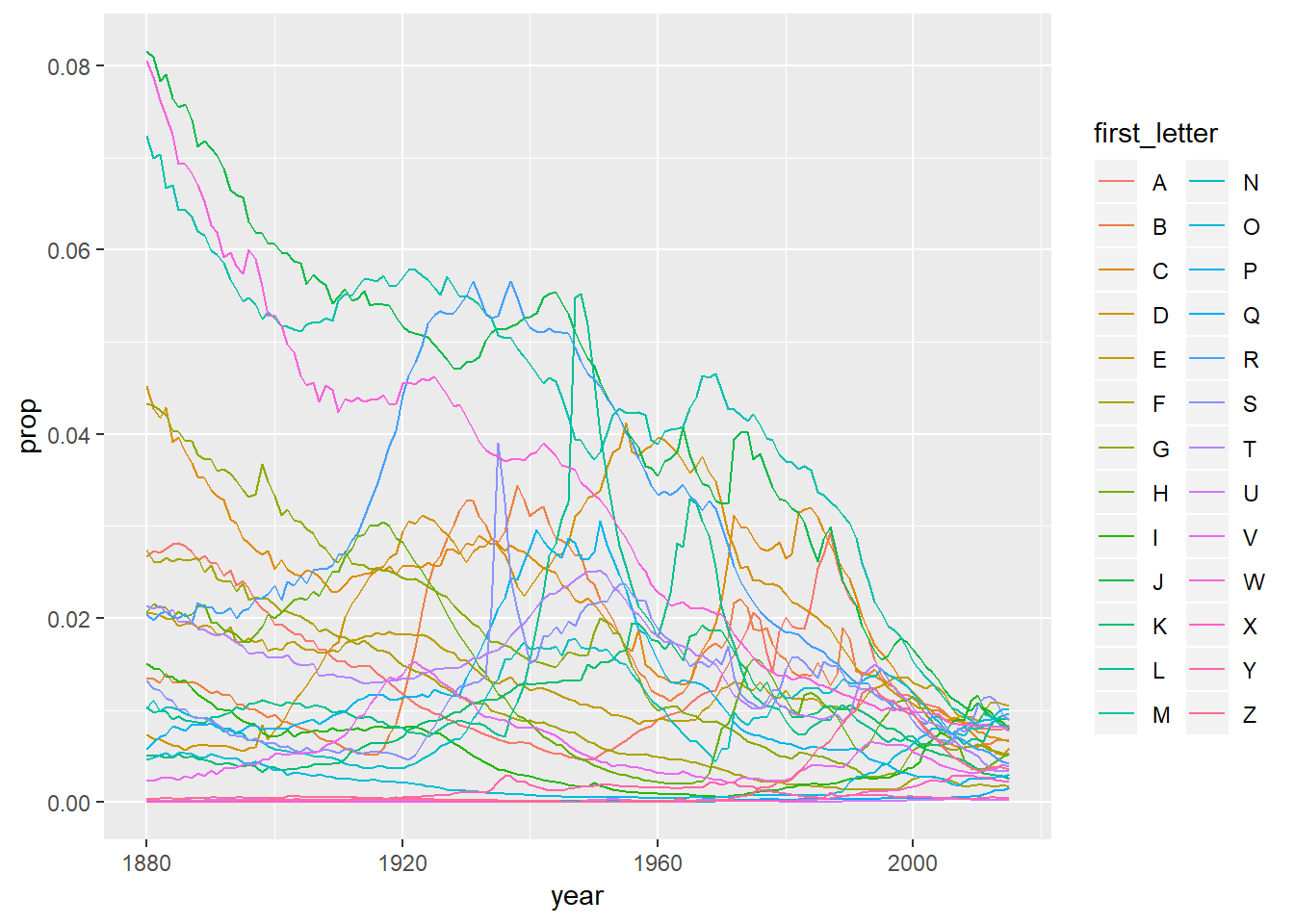
csv other example
The code below might be used to read csvs from a shared drive. I added on the ‘file_path_pull’ and ‘files_example’ components to add in information on the file paths and other details that were relevant. You might also add this data into a new column on the output…
files_path_pull <- dir("//companydomain.com/directory/",
                       pattern = "csv$",
                       full.names = TRUE)

files_example <- tibble(file_paths = files_path_pull[1:2]) %>%
  extract(file_paths, into = c("path", "name"), regex = "(.*)([0-9]{4}-[0-9]{2}-[0-9]{2})", remove = FALSE)

read_dir <- function(dir){
  #input vector of file paths name and output appended file
  out <- vector("list", length(dir))
  for (i in seq_along(out)){
    out[[i]] <- read_csv(dir[[i]])
  }
  out <-  bind_rows(out)
  out
}

read_dir(files_example$file_paths)
21.3.5.2 (with purrr)
purrr::map_lgl(iris, is.factor) %>%
  tibble::enframe()
## # A tibble: 5 x 2
## name value
## <chr> <lgl>
## 1 Sepal.Length FALSE
## 2 Sepal.Width FALSE
## 3 Petal.Length FALSE
## 4 Petal.Width FALSE
## 5 Species TRUESlightly less attractive printing
show_mean2 <- function(df) {
  df %>%
    keep(is.numeric) %>%
    map_dbl(mean, na.rm = TRUE)
}

show_mean2(flights)
## year month day dep_time sched_dep_time
## 2013.000000 6.548510 15.710787 1349.109947 1344.254840
## dep_delay arr_time sched_arr_time arr_delay flight
## 12.639070 1502.054999 1536.380220 6.895377 1971.923620
## air_time distance hour minute
## 150.686460 1039.912604 13.180247 26.230100Maybe slightly better printing and in df
show_mean3 <- function(df){
  df %>%
    keep(is.numeric) %>%
    map_dbl(mean, na.rm = TRUE) %>%
    as_tibble() %>%
    mutate(names = row.names(.))
}

show_mean3(flights)
## Warning: Calling `as_tibble()` on a vector is discouraged, because the behavior is likely to change in the future. Use `enframe(name = NULL)` instead.
## This warning is displayed once per session.## # A tibble: 14 x 2
## value names
## <dbl> <chr>
## 1 2013 1
## 2 6.55 2
## 3 15.7 3
## 4 1349. 4
## 5 1344. 5
## 6 12.6 6
## 7 1502. 7
## 8 1536. 8
## 9 6.90 9
## 10 1972. 10
## 11 151. 11
## 12 1040. 12
## 13 13.2 13
## 14 26.2 14Other method is to take advantage of the gather() function
flights %>%
  keep(is.numeric) %>%
  map(mean, na.rm = TRUE) %>%
  as_tibble() %>%
  gather()
## # A tibble: 14 x 2
## key value
## <chr> <dbl>
## 1 year 2013
## 2 month 6.55
## 3 day 15.7
## 4 dep_time 1349.
## 5 sched_dep_time 1344.
## 6 dep_delay 12.6
## 7 arr_time 1502.
## 8 sched_arr_time 1536.
## 9 arr_delay 6.90
## 10 flight 1972.
## 11 air_time 151.
## 12 distance 1040.
## 13 hour 13.2
## 14 minute 26.221.9.3.1
- mine can’t handle shortcut formulas or new functions
z <- sample(10)
z %>%
  every( ~ . < 11)
## [1] TRUE# e.g. below would fail
# z %>%
# every_loop( ~ . < 11)21.9 mirroring keep
below is one method for passing multiple, more complex arguments through keep, though you can also use function shortcuts (
~) inkeepanddiscard##how to pass multiple functions through keep? #can use map to subset columns by multiple criteria and then subset at end flights %>% purrr::map(is.na) %>% purrr::map_dbl(sum) %>% purrr::map_lgl(~.>10) %>% flights[.]## # A tibble: 336,776 x 6 ## dep_time dep_delay arr_time arr_delay tailnum air_time ## <int> <dbl> <int> <dbl> <chr> <dbl> ## 1 517 2 830 11 N14228 227 ## 2 533 4 850 20 N24211 227 ## 3 542 2 923 33 N619AA 160 ## 4 544 -1 1004 -18 N804JB 183 ## 5 554 -6 812 -25 N668DN 116 ## 6 554 -4 740 12 N39463 150 ## 7 555 -5 913 19 N516JB 158 ## 8 557 -3 709 -14 N829AS 53 ## 9 557 -3 838 -8 N593JB 140 ## 10 558 -2 753 8 N3ALAA 138 ## # ... with 336,766 more rows
invoke examples
Let’s change the example to be with quantile…
invoke(runif, n = 10)## [1] 0.775555937 0.328805817 0.920314980 0.176599637 0.210958651
## [6] 0.890200325 0.456075735 0.498955991 0.148438198 0.001021321list("01a", "01b") %>%
invoke(paste, ., sep = "-")## [1] "01a-01b"set.seed(123)
invoke_map(list(runif, rnorm), list(list(n = 10), list(n = 5)))## [[1]]
## [1] 0.2875775 0.7883051 0.4089769 0.8830174 0.9404673 0.0455565 0.5281055
## [8] 0.8924190 0.5514350 0.4566147
##
## [[2]]
## [1] 1.7150650 0.4609162 -1.2650612 -0.6868529 -0.4456620set.seed(123)
invoke_map(list(runif, rnorm), list(list(n = 10), list(5, 50)))## [[1]]
## [1] 0.2875775 0.7883051 0.4089769 0.8830174 0.9404673 0.0455565 0.5281055
## [8] 0.8924190 0.5514350 0.4566147
##
## [[2]]
## [1] 51.71506 50.46092 48.73494 49.31315 49.55434list(m1 = mean, m2 = median) %>% invoke_map(x = rcauchy(100))## $m1
## [1] 0.7316016
##
## $m2
## [1] 0.1690467rcauchy(100)## [1] -1.99514216 1.57378677 1.44901985 0.82604308 2.30072052
## [6] -0.04961749 0.52626840 0.29408692 0.47790231 -1.47138470
## [11] -2.54305059 -0.35508248 -1.65511601 -1.08467708 -15.03813728
## [16] -1.82118206 -0.62669137 -0.79456204 -0.06347636 5.19179251
## [21] 1.48851593 3.42095041 0.03289526 0.65171559 -0.53864091
## [26] 0.88812626 0.93375555 0.24570517 0.97348569 -1.11905466
## [31] -0.51964526 128.72537963 2.72138263 0.97793363 0.36391811
## [36] 2.77745450 -4.34935786 0.81096079 5.70518746 0.81669440
## [41] -138.41947905 2.02359725 -1.96283674 2.40809060 2.04850398
## [46] -9.41347275 -1.06265274 0.83312509 3.55625549 1.10375978
## [51] -2.31140048 0.65162145 -0.45665528 -1.02179975 -1.71189590
## [56] -2.57239721 2.35617831 -10.63750166 -0.41538322 -3.80770683
## [61] -0.55070513 1.49607830 -1.30359005 1.09910916 -3.27457763
## [66] 16.99304208 1.09921270 -4.86030197 -0.27969649 -0.31842181
## [71] 1.16466121 1.59209243 -0.04514112 -2.52586678 -0.19951960
## [76] 9.47599952 3.31841045 -1.82945785 0.51884667 -4.29179059
## [81] 0.93155898 -0.11880720 -3.03333758 -21.16294537 3.16450655
## [86] -0.39503234 2.19801293 1.27457150 0.59413768 0.60064481
## [91] 17.70703023 1.01880490 0.80764382 -1.63905090 0.15086898
## [96] -1.36865319 1.99173761 3.39988162 -0.63043489 -0.26058630Let’s store everything in a dataframe…
set.seed(123)
tibble(funs = list(rn = "rnorm", rp = "rpois", ru = "runif"),
       params = list(list(n = 20, mean = 10), list(n = 20, lambda = 3), list(n = 20, min = -1, max = 1))) %>%
  with(invoke_map_df(funs, params))
## # A tibble: 20 x 3
## rn rp ru
## <dbl> <int> <dbl>
## 1 9.44 1 0.330
## 2 9.77 2 -0.810
## 3 11.6 2 -0.232
## 4 10.1 2 -0.451
## 5 10.1 1 0.629
## 6 11.7 1 -0.103
## 7 10.5 2 0.620
## 8 8.73 3 0.625
## 9 9.31 2 0.589
## 10 9.55 5 -0.120
## 11 11.2 0 0.509
## 12 10.4 3 0.258
## 13 10.4 4 0.420
## 14 10.1 1 -0.999
## 15 9.44 3 -0.0494
## 16 11.8 2 -0.560
## 17 10.5 1 -0.240
## 18 8.03 4 0.226
## 19 10.7 5 -0.296
## 20 9.53 2 -0.778map_df(iris, ~.x*2)## Warning in Ops.factor(.x, 2): '*' not meaningful for factors## # A tibble: 150 x 5
## Sepal.Length Sepal.Width Petal.Length Petal.Width Species
## <dbl> <dbl> <dbl> <dbl> <lgl>
## 1 10.2 7 2.8 0.4 NA
## 2 9.8 6 2.8 0.4 NA
## 3 9.4 6.4 2.6 0.4 NA
## 4 9.2 6.2 3 0.4 NA
## 5 10 7.2 2.8 0.4 NA
## 6 10.8 7.8 3.4 0.8 NA
## 7 9.2 6.8 2.8 0.6 NA
## 8 10 6.8 3 0.4 NA
## 9 8.8 5.8 2.8 0.4 NA
## 10 9.8 6.2 3 0.2 NA
## # ... with 140 more rowsselect(iris, -Species) %>%
flatten_dbl() %>%
mean()## [1] 3.4645mean.and.median <- function(x){
list(mean = mean(x, na.rm = TRUE),
median = median(x, na.rm = TRUE))
}Difference between dfr and dfc, taken from here: https://bio304-class.github.io/bio304-fall2017/control-flow-in-R.html
iris %>%
  select(-Species) %>%
  map_dfr(mean.and.median) %>%
  bind_cols(tibble(names = names(select(iris, -Species))))
## # A tibble: 4 x 3
## mean median names
## <dbl> <dbl> <chr>
## 1 5.84 5.8 Sepal.Length
## 2 3.06 3 Sepal.Width
## 3 3.76 4.35 Petal.Length
## 4 1.20 1.3 Petal.Widthiris %>%
select(-Species) %>%
map_dfr(mean.and.median) %>%
bind_cols(tibble(names = names(select(iris, -Species))))## # A tibble: 4 x 3
## mean median names
## <dbl> <dbl> <chr>
## 1 5.84 5.8 Sepal.Length
## 2 3.06 3 Sepal.Width
## 3 3.76 4.35 Petal.Length
## 4 1.20 1.3 Petal.Widthiris %>%
select(-Species) %>%
map_dfc(mean.and.median)## # A tibble: 1 x 8
## mean median mean1 median1 mean2 median2 mean3 median3
## <dbl> <dbl> <dbl> <dbl> <dbl> <dbl> <dbl> <dbl>
## 1 5.84 5.8 3.06 3 3.76 4.35 1.20 1.3indexing nms caution
When creating your empty list, use indexes rather than names if you are creating values, otherwise you are creating new values on the list. E.g. in the example below I the output ends up being length 6 because you have the 3 NULL values plus the 3 newly created named positions.
x <- list(a = 1:10, b = 11:18, c = 19:25)
output <- vector("list", length(x))
for (nm in names(x)) {
  output[[nm]] <- x[[nm]] * 3
}
output
## [[1]]
## NULL
##
## [[2]]
## NULL
##
## [[3]]
## NULL
##
## $a
## [1] 3 6 9 12 15 18 21 24 27 30
##
## $b
## [1] 33 36 39 42 45 48 51 54
##
## $c
## [1] 57 60 63 66 69 72 75in-class notes
the map_* functions are essentially like running a flatten_* after running map. E.g. the two things below are equivalent
map(flights, typeof) %>%
  flatten_chr()
## [1] "integer" "integer" "integer" "integer" "integer"
## [6] "double" "integer" "integer" "double" "character"
## [11] "integer" "character" "character" "character" "double"
## [16] "double" "double" "double" "double"map_chr(flights, typeof)## year month day dep_time sched_dep_time
## "integer" "integer" "integer" "integer" "integer"
## dep_delay arr_time sched_arr_time arr_delay carrier
## "double" "integer" "integer" "double" "character"
## flight tailnum origin dest air_time
## "integer" "character" "character" "character" "double"
## distance hour minute time_hour
## "double" "double" "double" "double"Calculate the number of unique values for each level
iris %>%
  map(unique) %>%
  map_dbl(length)

map_int(iris, ~length(unique(.x)))
Iterate through different min and max values
min_params <- c(-1, 0, -10)
max_params <- c(11:13)
map2(.x = min_params, .y = max_params, ~runif(n = 10, min = .x, max = .y))
## [[1]]
## [1] 1.9234337 7.0166670 4.0117614 8.4583500 0.2343757 4.2187129
## [7] 10.8194838 9.7166134 9.6376287 1.1006318
##
## [[2]]
## [1] 1.568348 7.837223 4.122198 7.881098 3.844479 2.252293 9.387532
## [8] 1.123140 5.601348 6.138066
##
## [[3]]
## [1] 3.7997461 -2.3450586 1.2380998 11.9528980 1.1067551 10.4780551
## [7] 11.0320783 4.0009046 -0.5541351 -6.6168221When using pmap it’s often best to keep the parameters in a dataframe
min_df_params <- tibble(n = c(10, 15, 20, 50 ),
                        min = c(-1, 0, 1, 2),
                        max = c(0, 1, 2, 3))

pmap(min_df_params, runif)
## [[1]]
## [1] -0.06470020 -0.69877110 -0.93927943 -0.05227306 -0.27940373
## [6] -0.85770570 -0.45071534 -0.04590876 -0.41451665 -0.59548972
##
## [[2]]
## [1] 0.6478935 0.3198206 0.3077200 0.2197676 0.3694889 0.9842192 0.1542023
## [8] 0.0910440 0.1419069 0.6900071 0.6192565 0.8913941 0.6729991 0.7370777
## [15] 0.5211357
##
## [[3]]
## [1] 1.659838 1.821805 1.786282 1.979822 1.439432 1.311702 1.409475
## [8] 1.010467 1.183850 1.842729 1.231162 1.239100 1.076691 1.245724
## [15] 1.732135 1.847453 1.497527 1.387909 1.246449 1.111096
##
## [[4]]
## [1] 2.389994 2.571935 2.216893 2.444768 2.217991 2.502300 2.353905
## [8] 2.649985 2.374714 2.355445 2.533688 2.740334 2.221103 2.412746
## [15] 2.265687 2.629973 2.183828 2.863644 2.746568 2.668285 2.618018
## [22] 2.372238 2.529836 2.874682 2.581750 2.839768 2.312448 2.708290
## [29] 2.265018 2.594343 2.481290 2.265033 2.564590 2.913188 2.901874
## [36] 2.274167 2.321483 2.985641 2.619993 2.937314 2.466533 2.406833
## [43] 2.659230 2.152347 2.572867 2.238726 2.962359 2.601366 2.515030
## [50] 2.402573You can often use map a bunch of output that can then be stored in a tibble
tibble(type = map_chr(mtcars, typeof),
       means = map_dbl(mtcars, mean),
       median = map_dbl(mtcars, median),
       names = names(mtcars))
## # A tibble: 11 x 4
## type means median names
## <chr> <dbl> <dbl> <chr>
## 1 double 20.1 19.2 mpg
## 2 double 6.19 6 cyl
## 3 double 231. 196. disp
## 4 double 147. 123 hp
## 5 double 3.60 3.70 drat
## 6 double 3.22 3.32 wt
## 7 double 17.8 17.7 qsec
## 8 double 0.438 0 vs
## 9 double 0.406 0 am
## 10 double 3.69 4 gear
## 11 double 2.81 2 carbProvide the number of unique values for all columns excluding columns with numeric types or date types.
num_unique <- function(df) {
  df %>%
  keep(~is_character(.x) | is.factor(.x)) %>%
  map(~length(unique(.x))) %>%
  as_tibble() %>%
  gather() %>%
  rename(field_name = key, num_unique = value)
}

num_unique(flights)
## # A tibble: 4 x 2
## field_name num_unique
## <chr> <int>
## 1 carrier 16
## 2 tailnum 4044
## 3 origin 3
## 4 dest 105num_unique(iris)## # A tibble: 1 x 2
## field_name num_unique
## <chr> <int>
## 1 Species 3num_unique(mpg)## # A tibble: 6 x 2
## field_name num_unique
## <chr> <int>
## 1 manufacturer 15
## 2 model 38
## 3 trans 10
## 4 drv 3
## 5 fl 5
## 6 class 7This is a very powerful practice because it allows you to save / keep track of your manipulations and apply them at other locations, while keeping the logic very well organized – go and use this for documenting your work / transformations↩