Ch. 19: Functions
Key questions:
- 19.3.1. #1
- 19.4.4. #2, 3
- 19.5.5. #2 (actually make a function that fixes this)
function_name <- function(input1, input2) {}if () {}else if () {}else {}||(or) ,&&(and) – used to combine multiple logical expressions|and&are vectorized operations not to be used withifstatementsanychecks if any values in vector areTRUEallchecks if all values in vector areTRUEidenticalstrict check for if values are the samedplyr::nearfor more lenient comparison and typically better thanidenticalas unaffected by floating point numbers and fine with different typesswitchevaluate selected code based on position or name (good for replacing long chain ofifstatements). e.g.
Operation_Times2 <- function(x, y, op){
   first_op <- switch(op,
     plus = x + y,
     minus = x - y,
     times = x * y,
     divide = x / y,
     stop("Unknown op!")
   )

   first_op * 2
  }

Operation_Times2(5, 7, "plus")
## [1] 24stopstops expression and executes error action, note that.calldefault isFALSEwarninggenerates a warning that corresponds with arguments,suppressWarningsmay also be useful to nostopifnottest multiple args and will produce error message if any are not true – compromise that prevents you from tedious work of putting multipleif(){} else stop()statements...useful catch-all if your function primarily wraps another function (note that misspelled arguments will not raise an error), e.g.
commas <- function(...) stringr::str_c(..., collapse = ", ")
commas(letters[1:10])
## [1] "a, b, c, d, e, f, g, h, i, j"cutcan be used to discretize continuous variables (also saves longifstatements)returnallows you to return the function early, typically reserve use for when the function can return early with a simpler functioncatfunction to print label in outputinvisibleinput does not get printed out
19.2: When should you write a function?
19.2.1
Why is
TRUEnot a parameter torescale01()? What would happen ifxcontained a single missing value, andna.rmwasFALSE?TRUEdoesn’t change between uses.- The output would be
NA
In the second variant of
rescale01(), infinite values are left unchanged. Rewriterescale01()so that-Infis mapped to 0, andInfis mapped to 1.rescale01_inf <- function(x){ rng <- range(x, na.rm = TRUE, finite = TRUE) x_scaled <- (x - rng[1]) / (rng[2] - rng[1]) is_inf <- is.infinite(x) is_less0 <- x < 0 x_scaled[is_inf & is_less0] <- 0 x_scaled[is_inf & (!is_less0)] <- 1 x_scaled } x <- c(Inf, -Inf, 0, 3, -5) rescale01_inf(x)## [1] 1.000 0.000 0.625 1.000 0.000Practice turning the following code snippets into functions. Think about what each function does. What would you call it? How many arguments does it need? Can you rewrite it to be more expressive or less duplicative?
mean(is.na(x)) x / sum(x, na.rm = TRUE) sd(x, na.rm = TRUE) / mean(x, na.rm = TRUE)- See solutions below:
x <- c(1, 4, 2, 0, NA, 3, NA)

#mean(is.na(x))
perc_na <- function(x) {
  is.na(x) %>% mean()
}

perc_na(x)
## [1] 0.2857143#x / sum(x, na.rm = TRUE) prop_weighted <- function(x) { x / sum(x, na.rm = TRUE) } prop_weighted(x)## [1] 0.1 0.4 0.2 0.0 NA 0.3 NA#sd(x, na.rm = TRUE) / mean(x, na.rm = TRUE) CoefficientOfVariation <- function(x) { sd(x, na.rm = TRUE) / mean(x, na.rm = TRUE) } CoefficientOfVariation(x)## [1] 0.7905694Follow http://nicercode.github.io/intro/writing-functions.html to write your own functions to compute the variance and skew of a numeric vector.
- Re-do below to write measures for skew and variance (e.g. kurtosis, etc.)
var_bry <- function(x){
  sum((x - mean(x)) ^ 2) / (length(x) - 1)
}

skewness_bry <- function(x) {
  mean((x - mean(x)) ^ 3) / var_bry(x) ^ (3 / 2)
}
Let’s create some samples of distributions – normal, t (with 7 degrees of freedom), unifrom, poisson (with lambda of 2).
Note that an example with a cauchy distribution and looking at difference in kurtosis between that and a normal distribution has been moved to the Appendix section 19.2.1.4.
nd <- rnorm(10000)
td_df7 <- rt(10000, df = 7)
ud <- runif(10000)
pd_l2 <- rpois(10000, 2)
Verify that these functions match with established functions
dplyr::near(skewness_bry(pd_l2), e1071::skewness(pd_l2, type = 3))## [1] TRUEdplyr::near(var_bry(pd_l2), var(pd_l2))## [1] TRUELet’s look at the distributions as well as their variance an skewness
distributions_df <- tibble(normal_dist = nd,
       t_7df_dist = td_df7,
       uniform_dist = ud,
       poisson_dist = pd_l2)

distributions_df %>%
  gather(normal_dist:poisson_dist, value = "sample", key = "dist_type") %>%
  mutate(dist_type = factor(forcats::fct_inorder(dist_type))) %>%
  ggplot(aes(x = sample))+
  geom_histogram()+
  facet_wrap(~ dist_type, scales = "free")
## `stat_bin()` using `bins = 30`. Pick better value with `binwidth`.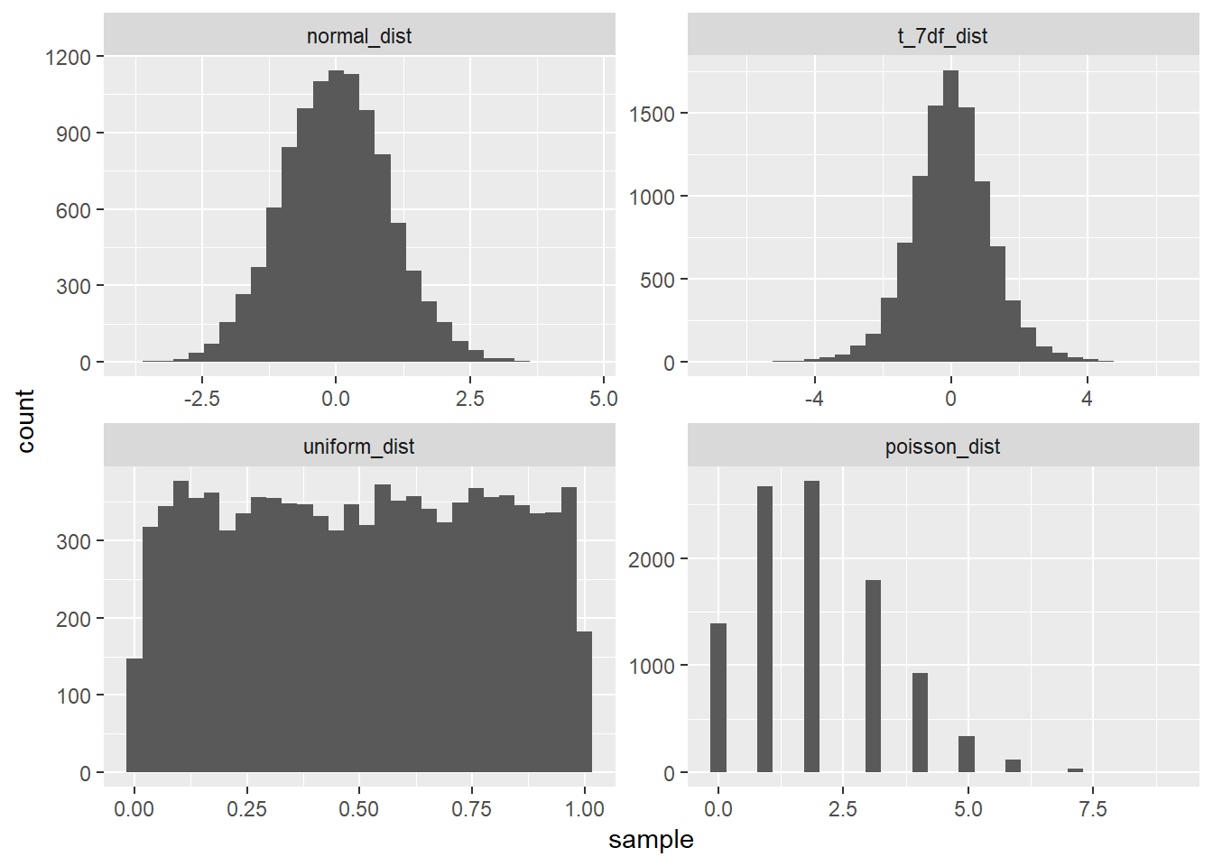
tibble(dist_type = names(distributions_df),
skewness = purrr::map_dbl(distributions_df, skewness_bry),
variance = purrr::map_dbl(distributions_df, var_bry))
## # A tibble: 4 x 3 ## dist_type skewness variance ## <chr> <dbl> <dbl> ## 1 normal_dist 0.0561 0.988 ## 2 t_7df_dist -0.0263 1.40 ## 3 uniform_dist -0.00678 0.0833 ## 4 poisson_dist 0.680 1.98- excellent video explaining intuition behind skewness: https://www.youtube.com/watch?v=z3XaFUP1rAM
Write
both_na(), a function that takes two vectors of the same length and returns the number of positions that have anNAin both vectors.both_na <- function(x, y) { if (length(x) == length(y)) { sum(is.na(x) & is.na(y)) } else stop("Vectors are not equal length") } x <- c(4, NA, 7, NA, 3) y <- c(NA, NA, 5, NA, 0) z <- c(NA, 4) both_na(x, y)## [1] 2both_na(x, z)## Error in both_na(x, z): Vectors are not equal lengthWhat do the following functions do? Why are they useful even though they are so short?
is_directory <- function(x) file.info(x)$isdir is_readable <- function(x) file.access(x, 4) == 0- first checks if what is being referred to is actually a directory
- second checks if a specific file is readable
Read the complete lyrics to “Little Bunny Foo Foo”. There’s a lot of duplication in this song. Extend the initial piping example to recreate the complete song, and use functions to reduce the duplication.
19.3: Functions are for humans and computers
- Recommends snake_case over camelCase, but just choose one and be consistent
- When functions have a link, common prefix over suffix (i.e. input_select, input_text over, select_input, text_input)
- ctrl + shift + r creates section breaks in R scripts like below
# test label --------------------------------------------------------------
- (though these cannot be made in markdown documents)
19.3.1
Read the source code for each of the following three functions, puzzle out what they do, and then brainstorm better names.
f1 <- function(string, prefix) { substr(string, 1, nchar(prefix)) == prefix } f2 <- function(x) { if (length(x) <= 1) return(NULL) x[-length(x)] } f3 <- function(x, y) { rep(y, length.out = length(x)) }f1:check_prefixf2:return_not_lastf3:repeat_for_length
Take a function that you’ve written recently and spend 5 minutes brainstorming a better name for it and its arguments.
- done seperately
Compare and contrast
rnorm()andMASS::mvrnorm(). How could you make them more consistent?- uses mu = and Sigma = instead of mean = and sd = , and has extra parameters like tol, empirical, EISPACK
- Similar in that both are pulling samples from gaussian distribution
mvrnormis multivariate though, could change name tornorm_mv
Make a case for why
norm_r(),norm_d()etc would be better thanrnorm(),dnorm(). Make a case for the opposite.norm_*would show the commonality of them being from the same distribution. One could argue the important commonality though may be more related to it being either a random sample or a density distribution, in which case ther*ord*coming first may make more sense. To me, the fact that the help pages has all of the ‘normal distribution’ functions on the same page suggests the former may make more sense. However, I actually like having it be set-up the way it is, because I am more likely to forget the name of the distribution type I want over the fact that I want a random sample, so it’s easier to typerand then do ctrl + space and have autocomplete help me find the specific distribution I want, e.g.rnorm,runif,rpois,rbinom…
19.4: Conditional execution
Function example that uses if statement:
has_name <- function(x) {
  nms <- names(x)
  if (is.null(nms)) {
    rep(FALSE, length(x))
  } else {
    !is.na(nms) & nms != ""
  }
}- note that if all names are blank, it returns the one-unit vector value
NULL, hence the need for theifstatement here…33
19.4.4.
What’s the difference between
ifandifelse()? Carefully read the help and construct three examples that illustrate the key differences.ifelseis vectorized,ifis not- Typically use
ifin functions when giving conditional options for how to evaluate - Typically use
ifelsewhen changing specific values in a vector
- Typically use
- If you supply
ifwith a vector of length > 1, it will use the first value
x <- c(3, 4, 6)
y <- c("5", "c", "9")

# Use `ifelse` simple transformations of values
ifelse(x < 5, 0, x)
## [1] 0 0 6# Use `if` for single condition tests cutoff_make0 <- function(x, cutoff = 0){ if(is.numeric(x)){ ifelse(x < cutoff, 0, x) } else stop("The input provided is not a numeric vector") } cutoff_make0(x, cutoff = 4)## [1] 0 4 6cutoff_make0(y, cutoff = 4)## Error in cutoff_make0(y, cutoff = 4): The input provided is not a numeric vectorWrite a greeting function that says “good morning”, “good afternoon”, or “good evening”, depending on the time of day. (Hint: use a time argument that defaults to
lubridate::now(). That will make it easier to test your function.)greeting <- function(when) { time <- hour(when) if (time < 12 && time > 4) { greating <- "good morning" } else if (time < 17 && time >= 12) { greeting <- "good afternoon" } else greeting <- "good evening" when_char <- as.character(when) mid <- ", it is: " cat(greeting, mid, when_char, sep = "") } greeting(now())## good evening, it is: 2019-06-05 19:28:02Implement a
fizzbuzzfunction. It takes a single number as input. If the number is divisible by three, it returns “fizz”. If it’s divisible by five it returns “buzz”. If it’s divisible by three and five, it returns “fizzbuzz”. Otherwise, it returns the number. Make sure you first write working code before you create the function.fizzbuzz <- function(x){ if(is.numeric(x) && length(x) == 1){ y <- "" if (x %% 5 == 0) y <- str_c(y, "fizz") if (x %% 3 == 0) y <- str_c(y, "buzz") if (str_length(y) == 0) { print(x) } else print(y) } else stop("Input is not a numeric vector with length 1") } fizzbuzz(4)## [1] 4fizzbuzz(10)## [1] "fizz"fizzbuzz(6)## [1] "buzz"fizzbuzz(30)## [1] "fizzbuzz"fizzbuzz(c(34, 21))## Error in fizzbuzz(c(34, 21)): Input is not a numeric vector with length 1How could you use
cut()to simplify this set of nested if-else statements?if (temp <= 0) { "freezing" } else if (temp <= 10) { "cold" } else if (temp <= 20) { "cool" } else if (temp <= 30) { "warm" } else { "hot" }- Below is example of fix
temp <- seq(-10, 50, 5)
cut(temp,
    breaks = c(-Inf, 0, 10, 20, 30, Inf),  #need to include negative and positive infiniity
    labels = c("freezing", "cold", "cool", "warm", "hot"),
    right = TRUE,
    oredered_result = TRUE)
## [1] freezing freezing freezing cold cold cool cool ## [8] warm warm hot hot hot hot ## Levels: freezing cold cool warm hotHow would you change the call to
cut()if I’d used<instead of<=? What is the other chief advantage ofcut()for this problem? (Hint: what happens if you have many values intemp?)- See below change to
rightargument
cut(temp,
    breaks = c(-Inf, 0, 10, 20, 30, Inf),  #need to include negative and positive infiniity
    labels = c("freezing", "cold", "cool", "warm", "hot"),
    right = FALSE,
    oredered_result = TRUE)
## [1] freezing freezing cold cold cool cool warm ## [8] warm hot hot hot hot hot ## Levels: freezing cold cool warm hotWhat happens if you use
switch()with numeric values?- It will return the index of the argument.
- In example below, I input ‘3’ into
switchvalue so it does thetimesargument
- In example below, I input ‘3’ into
math_operation <- function(x, y, op){
   switch(op,
     plus = x + y,
     minus = x - y,
     times = x * y,
     divide = x / y,
     stop("Unknown op!")
   )
  }

math_operation(5, 4, 3)
## [1] 20- It will return the index of the argument.
What does this
switch()call do? What happens ifxis “e”?x <- "e" switch(x, a = , b = "ab", c = , d = "cd" )Experiment, then carefully read the documentation.
- If
xis ‘e’ nothing will be outputted. Ifxis ‘c’ or ‘d’ then ‘cd’ is outputted. If ‘a’ or ‘b’ then ‘ab’ is outputeed. If blank it will continue down list until reaching an argument to output.
- If
19.5: Function arguments
Common non-descriptive short argument names:
x,y,z: vectors.w: a vector of weights.df: a data frame.i,j: numeric indices (typically rows and columns).n: length, or number of rows.p: number of columns.
19.5.5.
What does
commas(letters, collapse = "-")do? Why?commasfunction is below
commas <- function(...) stringr::str_c(..., collapse = ", ")

commas(letters[1:10])
## [1] "a, b, c, d, e, f, g, h, i, j"commas(letters[1:10], collapse = "-")## Error in stringr::str_c(..., collapse = ", "): formal argument "collapse" matched by multiple actual arguments- The above fails because are essentially specifying two different values for the
collapseargument - Takes in vector of mulitple strings and outputs one-unit character string with items concatenated together and seperated by columns
- Is able to do this via use of
...that turns this into a wrapper onstringr::str_cwith thecollapsevalue specified
It’d be nice if you could supply multiple characters to the
padargument, e.g.rule("Title", pad = "-+"). Why doesn’t this currently work? How could you fix it?- current
rulefunction is below
rule <- function(..., pad = "-") {
  title <- paste0(...)
  width <- getOption("width") - nchar(title) - 5
  cat(title, " ", stringr::str_dup(pad, width), "\n", sep = "")
}

# Note that `cat` is used instead of `paste` because paste would output it as a character vector, whereas `cat` is focused on just ouptut, could also have used `print`, though print does more conversion than cat does (apparently)

rule("Tis the season"," to be jolly")
## Tis the season to be jolly --------------------------------------------- doesn’t work because pad ends-up being too many characters in this situation
rule("Tis the season"," to be jolly", pad="+-")## Tis the season to be jolly +-+-+-+-+-+-+-+-+-+-+-+-+-+-+-+-+-+-+-+-+-+-+-+-+-+-+-+-+-+-+-+-+-+-+-+-+-+-+-+-+-+-+-+-- instead would need to make the number of times
padis duplicated dependent on its length, see below for fix
rule_pad_fix <- function(..., pad = "-") {
  title <- paste0(...)
  width <- getOption("width") - nchar(title) - 5
  width_fix <- width %/% stringr::str_length(pad)
  cat(title, " ", stringr::str_dup(pad, width_fix), "\n", sep = "")
}

rule_pad_fix("Tis the season"," to be jolly", pad="+-")
## Tis the season to be jolly +-+-+-+-+-+-+-+-+-+-+-+-+-+-+-+-+-+-+-+-+-+-- current
What does the
trimargument tomean()do? When might you use it?trimspecifies proportion of data to take off from both ends, good with outliers
mean(c(-1000, 1:100, 100000), trim = .025)## [1] 50.5The default value for the
methodargument tocor()isc("pearson", "kendall", "spearman"). What does that mean? What value is used by default?- is showing that you can choose from any of these, will default to use
pearson(value in first position)
- is showing that you can choose from any of these, will default to use
19.6: Return values
show_missings <- function(df) {
  n <- sum(is.na(df))
  cat("Missing values: ", n, "\n", sep = "")
  invisible(df)
}

x <- show_missings(mtcars)
## Missing values: 0str(x)## 'data.frame': 32 obs. of 11 variables:
## $ mpg : num 21 21 22.8 21.4 18.7 18.1 14.3 24.4 22.8 19.2 ...
## $ cyl : num 6 6 4 6 8 6 8 4 4 6 ...
## $ disp: num 160 160 108 258 360 ...
## $ hp : num 110 110 93 110 175 105 245 62 95 123 ...
## $ drat: num 3.9 3.9 3.85 3.08 3.15 2.76 3.21 3.69 3.92 3.92 ...
## $ wt : num 2.62 2.88 2.32 3.21 3.44 ...
## $ qsec: num 16.5 17 18.6 19.4 17 ...
## $ vs : num 0 0 1 1 0 1 0 1 1 1 ...
## $ am : num 1 1 1 0 0 0 0 0 0 0 ...
## $ gear: num 4 4 4 3 3 3 3 4 4 4 ...
## $ carb: num 4 4 1 1 2 1 4 2 2 4 ...- can still use in pipes
mtcars %>%
  show_missings() %>%
  mutate(mpg = ifelse(mpg < 20, NA, mpg)) %>%
  show_missings()
## Missing values: 0
## Missing values: 18Appendix
19.2.1.4
Function for Standard Error:
x <- c(5, -2, 8, 6, 9)
sd(x, na.rm = TRUE) / sqrt(sum(!is.na(x)))
## [1] 1.933908sample_se <- function(x) {
sd(x, na.rm = TRUE) / sqrt(sum(!is.na(x)) - 1)
}
#sqrt(var(x)/sum(!is.na(x)))
sample_se(x)## [1] 2.162175Function for kurtosis:
kurtosis_type3 <- function(x){
  sum((x - mean(x)) ^ 4) / length(x) / sd(x) ^ 4 - 3
}
Notice differences between cauchy and normal distribution
set.seed(1235)
norm_exp <- rnorm(10000)

set.seed(1235)
cauchy_exp <- rcauchy(10000)hist(norm_exp)
hist(cauchy_exp)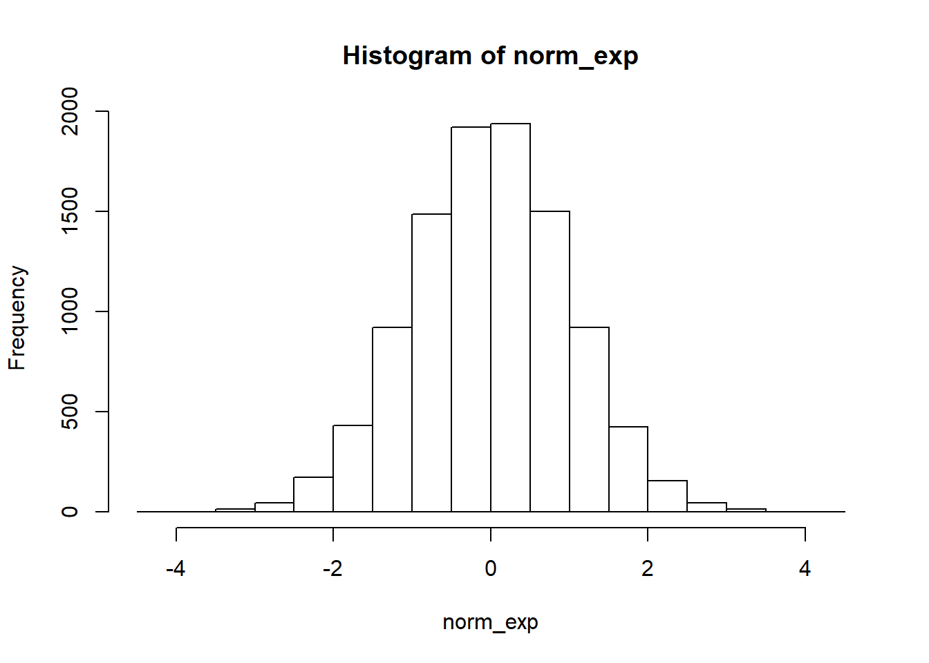
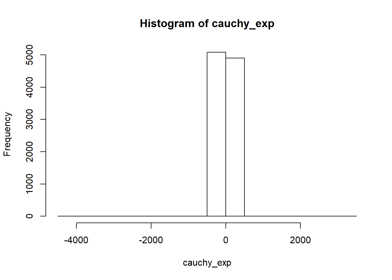
kurtosis
kurtosis_type3(norm_exp)## [1] 0.06382172kurtosis_type3(cauchy_exp)## [1] 1197.05219.2.3.5
position_both_na <- function(x, y) {
  if (length(x) == length(y)) {
  (c(1:length(x)))[(is.na(x) & is.na(y))]
  } else
  stop("Vectors are not equal length")
}

x <- c(4, NA, 7, NA, 3)
y <- c(NA, NA, 5, NA, 0)
z <- c(NA, 4)
both_na(x, y)
## [1] 2both_na(x, z)## Error in both_na(x, z): Vectors are not equal length- specifies position where both are
NA - second example shows returning of ‘stop’ argument
NULLtypes are not vectors but only single length elements of a different type.is.nullis not vectorized in the way thatis.na. E.g. it’s job is to returnTRUEif given aNULL. For example, a list ofNULLs is alisttype (not aNULLtype) therefore the following:is.null(list(NULL, NULL))would beFALSE– to return a list ofTRUEvalues you would need to runmap(list(NULL, NULL), is.null).↩