Ch. 27: R Markdown

Functions and notes:

shortcut for inserting code chunk is cmd/ctrl+alt+i
shortcut for running entire code chunks: cmd/ctrl+shift+enter
chunk options
- chunk name is first part after type of code in chunk, e.g. code chunk by name: "```{r by-name}"
- eval = FALSE show example output code, but don’t evaluate
- include = FALSE evaluate code but don’t show code or output
- echo = FALSE is for when you just want the output but not the code itself
- message = FALSE or warning = False prevents messages or warnings appearing in the finished line
- error = TRUE causes code to render even if there is an error
- results = 'hide' hides printied output and fig.show = 'hide' hides plots
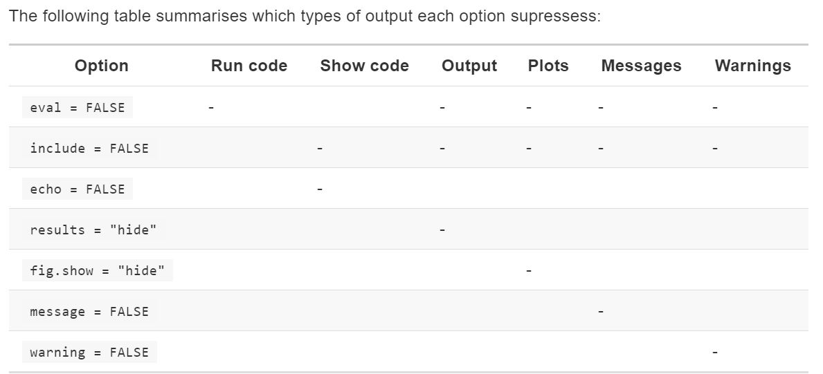
  - allows you to hide particular bits of output
- cache = TRUE save output of chunk to separate folder (speeds-up rendering)
- dependson = "chunk_name" update chunk if dependency changes
- cache.extra if output from function changes, will re-render – useful for if you only want to update if for example a file changes, e.g.

rawdata <- readr::read_csv("a_very_large_file.csv")

good idea to name code chunks after main object created
knitr::clean_cache clear out your caches

knitr::opts_chunk use to change knitting options

e.g.

# when writing books and tutorials
knitr::opts_chunk$set(
  comment = "#>",
  collapse = TRUE
)

# hiding code for report
knitr::opts_chunk$set(
  echo = FALSE
)
# may also set `message = FALSE` and `warning = FALSE`

rmarkdown::render programmatically knit documents
- e.g. rmarkdown::render("27-r-markdown.Rmd", output_format = "all") to render all formats in YAML header
knitr::kable to make dataframe more visible for printing when knitting
- also see xtable, stargazer, pander, tables, and ascii packages
format helpful when inserting numbers into texts, e.g.

comma <- function(x) format(x, digits = 2, big.mark = ",")
comma(3452345)

## [1] "3,452,345"

comma(.12358124331)

## [1] "0.12"

Use params: in YAML header to add in specific values or create parameterized reports, e.g.

params:
  start: !r lubridate::ymd("2015-01-01")
  snapshot: !r lubridate::ymd_hms("2015-01-01 12:30:00")

Full chunk options here: https://yihui.name/knitr/options/

27.2 R Markdown basics

27.2.1

Create a new notebook using File > New File > R Notebook. Read the instructions. Practice running the chunks. Verify that you can modify the code, re-run it, and see modified output.

Done seperately.
Create a new R Markdown document with File > New File > R Markdown… Knit it by clicking the appropriate button. Knit it by using the appropriate keyboard short cut. Verify that you can modify the input and see the output update.

Done seperately.
Compare and contrast the R notebook and R markdown files you created above. How are the outputs similar? How are they different? How are the inputs similar? How are they different? What happens if you copy the YAML header from one to the other?
- Both by default have code chunks display ‘in-line’ while working, though with RMD can force to not output in-line.
- When rendering, default of notebooks will be to render whichever chunks have been rendered during interactive session, whereas RMD document needs directions from code chunk options
  - I generally prefer .Rmd files to notebooks.⁴⁶
Create one new R Markdown document for each of the three built-in formats: HTML, PDF and Word. Knit each of the three documents. How does the output differ? How does the input differ? (You may need to install LaTeX in order to build the PDF output — RStudio will prompt you if this is necessary.)

Done seperately. HTML does not have page numbers. Plots or other outputs with interactive components will often only be viewable from html (e.g. flexdashboard, plotly, …). Some input options will work across all formats, e.g. toc: true, however other options like code folding may be specific to a format, e.g. code folding will only work with html.

27.3: Text formatting with Markdown

Print file from Hadley’s github page with commmon formatting:

cat(readr::read_file("https://raw.githubusercontent.com/hadley/r4ds/master/rmarkdown/markdown.Rmd"))

Other notes The following will actually run in the console when knitted (and not in the knitted document):

summary(mpg)

27.3.1

Practice what you’ve learned by creating a brief CV. The title should be your name, and you should include headings for (at least) education or employment. Each of the sections should include a bulleted list of jobs/degrees. Highlight the year in bold.

this is a weak example (see __ for better examples):

Using the R Markdown quick reference, figure out how to:
Add a footnote.

Here is a foonote reference⁴⁷ and another⁴⁸ and a 3rd⁴⁹ and an in-line one⁵⁰

Add a horizontal rule.

A linked phrase.

pagebreaks above and below (AKA horizontal rules)

Add a block quote.

There is no spoon.
-The Matrix

Copy and paste the contents of diamond-sizes.Rmd from https://github.com/hadley/r4ds/tree/master/rmarkdown in to a local R markdown document. Check that you can run it, then add text after the frequency polygon that describes its most striking features.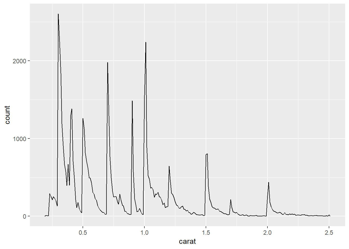

It’s interesting that the count of number of diamonds spikes at whole numbers…

27.4: Code chunks

27.4.7

Add a section that explores how diamond sizes vary by cut, colour, and clarity. Assume you’re writing a report for someone who doesn’t know R, and instead of setting echo = FALSE on each chunk, set a global option.
- put this into a code chunk:
```
knitr::opts_chunk$set(echo = FALSE)
```

Download diamond-sizes.Rmd from https://github.com/hadley/r4ds/tree/master/rmarkdown. Add a section that describes the largest 20 diamonds, including a table that displays their most important attributes.

diamonds %>% 
  filter(min_rank(-carat) <= 20) %>% 
  select(starts_with("c")) %>% 
  arrange(desc(carat)) %>% 
  knitr::kable(caption = "The four C's of the 20 biggest diamonds")

Table 1: The four C’s of the 20 biggest diamonds
carat	cut	color	clarity
5.01	Fair	J	I1
4.50	Fair	J	I1
4.13	Fair	H	I1
4.01	Premium	I	I1
4.01	Premium	J	I1
4.00	Very Good	I	I1
3.67	Premium	I	I1
3.65	Fair	H	I1
3.51	Premium	J	VS2
3.50	Ideal	H	I1
3.40	Fair	D	I1
3.24	Premium	H	I1
3.22	Ideal	I	I1
3.11	Fair	J	I1
3.05	Premium	E	I1
3.04	Very Good	I	SI2
3.04	Premium	I	SI2
3.02	Fair	I	I1
3.01	Premium	I	I1
3.01	Premium	F	I1
3.01	Fair	H	I1
3.01	Premium	G	SI2
3.01	Ideal	J	SI2
3.01	Ideal	J	I1
3.01	Premium	I	SI2
3.01	Fair	I	SI2
3.01	Fair	I	SI2
3.01	Good	I	SI2
3.01	Good	I	SI2
3.01	Good	H	SI2
3.01	Premium	J	SI2
3.01	Premium	J	SI2

Modify diamonds-sizes.Rmd to use comma() to produce nicely formatted output. Also include the percentage of diamonds that are larger than 2.5 carats.
```
diamonds %>% 
  summarise(`proportion big` = (sum(carat > 2.5) / n()) %>% 
              comma()) %>% 
  knitr::kable()
```
proportion big

0.0023

proportion big
0.0023

Set up a network of chunks where d depends on c and b, and both b and c depend on a. Have each chunk print lubridate::now(), set cache = TRUE, then verify your understanding of caching.

lubridate::now()

## [1] "2019-06-05 19:31:49 EDT"

lubridate::now()

## [1] "2019-06-05 19:31:49 EDT"

lubridate::now()

## [1] "2019-06-05 19:31:50 EDT"

lubridate::now()

## [1] "2019-06-05 19:31:50 EDT"

Make sure the following packages are installed:

I’ve found some of my company’s security software sometimes acts-up when working interactively if I have my chunk output in-line (just slows down). Hence, I ‘uncheck’ Show output inline for all Rmarkdown documents from Tools–>Global Options –>Appearance.↩
Here is the foonote.↩
here’s one with multiple blocks.
boo ya this is an awesome foonote.
don’t you believe it!↩
and the third↩
Superb fourth footnote.↩